In this topic, we will focus on deep learning, a subfield of AI that has gained significant attention and has become the cornerstone of many state-of-the-art AI applications. Deep learning models have demonstrated exceptional capabilities in learning complex patterns and representations directly from raw data, leading to remarkable breakthroughs in various domains.
Throughout this topic, we will explore the relationship between deep learning and AI, understanding how deep learning fits into the broader landscape of artificial intelligence and its role in enabling machines to learn and make intelligent decisions.
Traditional machine learning refers to a set of algorithms and techniques that enable machines to learn from data and make predictions or decisions without explicit programming. In traditional machine learning, the focus is on extracting meaningful features from the input data and training models to learn patterns and relationships between the features and the target output.
Traditional machine learning algorithms are typically designed to solve specific tasks such as classification, regression, clustering, or dimensionality reduction. These algorithms rely on handcrafted features that are engineered by domain experts or data scientists. Feature engineering involves selecting, transforming, and combining relevant features from the input data to represent the underlying patterns and relationships.
Once the features are extracted, the machine learning model is trained using labelled data. During training, the model learns the relationships between the input features and the output by optimizing a specific objective or loss function. The trained model can then be used to make predictions or decisions on new, unseen data.
Watch the video below to find out more about traditional machine learning.
While traditional machine learning has achieved significant success in many applications, it relies heavily on human expertise in feature engineering and may struggle to handle complex and high-dimensional data. This limitation led to the emergence of deep learning.

Deep learning (DL) is a subfield of machine learning that focuses on training artificial neural networks with multiple layers, also known as deep neural networks, to learn and represent complex patterns and relationships directly from raw data. DL models are designed to automatically learn hierarchical representations, enabling them to capture intricate structures and extract high-level features from the input data.
DL has gained significant attention and importance due to several key factors:

- Representation learning: DL models excel at automatically learning feature representations from raw data. Unlike traditional machine learning approaches that rely on manual feature engineering, DL algorithms can discover and extract relevant features directly from the data, allowing for more efficient and accurate learning.
- Handling big data: DL models are particularly suited for big data applications. With the increasing availability of large-scale datasets, DL algorithms can leverage the abundance of data to learn complex patterns and make accurate predictions. DL's ability to scale with data makes it a powerful tool for extracting insights from massive datasets.
- Performance improvement: DL has demonstrated remarkable performance improvements in various domains. It has achieved state-of-the-art results in challenging tasks such as image recognition, natural language processing, speech recognition, and autonomous driving. DL models have shown the potential to surpass human-level performance in specific domains, leading to breakthroughs and advancements in AI.
- End-to-end learning: DL enables end-to-end learning, where the model learns to perform a task directly from the raw input to the desired output. This eliminates the need for manual feature engineering and simplifies the overall pipeline, making DL models more flexible and adaptable to different domains and tasks.
- Generalization and adaptability: DL models can generalize well to unseen data and adapt to different scenarios. They can capture intricate patterns and variations in the data, allowing for robust performance across diverse datasets. DL models can also be fine-tuned or transferred to related tasks or domains, leveraging the learned representations for improved performance in new contexts.
Overall, DL has revolutionized the field of AI by enabling machines to learn and reason in ways that mimic human intelligence. Its importance lies in its ability to tackle complex problems, handle massive amounts of data, and deliver superior performance across various domains. DL's potential to advance AI applications and solve real-world challenges makes it a crucial area of study and research.
DL is a subset of AI and represents one of the key methodologies within the broader field of AI. DL focuses on training deep neural networks with multiple layers to learn and represent complex patterns and relationships directly from raw data.
AI, on the other hand, is a broader concept that encompasses various techniques and approaches aimed at developing intelligent systems capable of performing tasks that typically require human intelligence. These tasks include speech recognition, image recognition, natural language processing, decision-making, and problem-solving.
DL plays a crucial role in AI by providing powerful tools and techniques for learning and extracting meaningful representations from data. It enables machines to automatically learn hierarchical features and patterns, allowing them to understand, interpret, and make predictions from complex data such as images, text, and audio.
DL has greatly advanced the field of AI by enabling breakthroughs in various areas, including computer vision, natural language processing, and speech recognition. With its ability to learn directly from raw data and automatically extract relevant features, DL has revolutionized many AI applications and achieved state-of-the-art performance in tasks that were previously challenging for traditional machine-learning approaches.
The relationship between DL and AI can be seen as follows:
- DL provides the tools and methodologies to solve complex AI tasks, making it an integral part of the AI landscape.
- As DL continues to advance, it plays a vital role in pushing the boundaries of what machines can achieve in terms of understanding and reasoning, thereby driving the overall progress of AI.
Watch the video below to find out more about AI, DL and machine learning.
The building blocks of deep learning refer to the fundamental components and concepts that form the foundation of deep neural networks, which are the core models used in deep learning. These building blocks include the following:
- Artificial neurons (nodes): Artificial neurons, also known as nodes or units, are the basic computational units of a neural network. They receive inputs, apply a mathematical operation to those inputs, and produce an output. Neurons are organized into layers, with each layer consisting of multiple neurons.
- Neural network architecture: The architecture of a neural network defines its structure, including the arrangement and connectivity of the neurons. Deep learning models typically have multiple hidden layers between the input and output layers, allowing them to learn hierarchical representations of the data.
- Activation functions: Activation functions introduce non-linearity to the output of each neuron, enabling neural networks to learn complex patterns and relationships. Common activation functions include the sigmoid function, hyperbolic tangent (tanh) function, and rectified linear unit (ReLU) function.
- Forward propagation: Forward propagation refers to the process of passing input data through the neural network to generate predictions or outputs. In this process, each neuron's output is computed based on the weighted sum of its inputs and the activation function.
- Backpropagation: Backpropagation is a key algorithm for training deep neural networks. It involves computing the gradient of the loss function with respect to the network's parameters (weights and biases) and updating the parameters using gradient descent optimization. Backpropagation enables the network to learn by iteratively adjusting its weights to minimize the difference between predicted outputs and the ground truth.
- Loss function: The loss function measures the discrepancy between the predicted outputs of the neural network and the actual targets. It quantifies the network's performance during training and guides the optimization process. Common loss functions include mean squared error (MSE), cross-entropy loss, and binary log loss.
- Optimization algorithms: Optimization algorithms are used to update the network's parameters during training. They determine the direction and magnitude of parameter updates based on the gradients computed through backpropagation. Popular optimization algorithms include stochastic gradient descent (SGD), Adam, and RMSprop.
- Regularization techniques: Deep learning models are prone to overfitting, where they perform well on training data but fail to generalize to new, unseen data. Regularization techniques such as L1 and L2 regularization, dropout, and early stopping are employed to prevent overfitting and improve the model's ability to generalize.
These building blocks form the basis of deep learning models and provide the necessary tools for learning complex patterns and representations from data. By combining these elements in various ways, deep learning models can effectively solve a wide range of tasks, including image classification, object detection, natural language processing, and speech recognition.
Watch the video below to find out more about deep learning.
A single-layer neural network, also known as a single-layer perceptron, is the simplest form of a neural network. It consists of only one layer of artificial neurons, where each neuron is connected directly to the input data. The output of the network is computed based on the weighted sum of the inputs, followed by an activation function.
In a single-layer neural network, the neurons have no hidden layers, which means that there are no intermediate layers of computation between the input and output. The weights associated with each neuron determine the strength of the connections between the input and the neuron's output. These weights are typically learned through a training process.
The activation function in a single-layer neural network introduces non-linearity to the output, allowing the network to learn non-linear relationships between the input and output. Common activation functions used in single-layer networks include the sigmoid function, which maps the weighted sum to a value between 0 and 1, and the step function, which produces binary outputs based on a threshold.
Single-layer neural networks are primarily used for binary classification tasks, where the network learns to separate input data into two distinct classes. They are limited in their ability to learn complex patterns and relationships in data since they lack the capability of modelling non-linear decision boundaries. However, they can still be effective for simple classification problems or as building blocks in more complex neural network architectures.
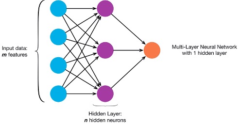
A multi-layer neural network, also known as a multi-layer perceptron (MLP), is a type of artificial neural network that consists of multiple layers of artificial neurons, including input, hidden, and output layers. Each layer is composed of multiple neurons, and the neurons are connected to the neurons in adjacent layers through weighted connections.
The key characteristic of a multi-layer neural network is its ability to learn and model complex patterns and relationships in data by introducing hidden layers. The hidden layers enable the network to learn hierarchical representations of the input data, where each layer learns increasingly abstract features and patterns. This hierarchical representation allows the network to capture and understand intricate relationships within the data.
In a multi-layer neural network, the input layer receives the raw input data, which could be features or pixels of an image, attributes of a dataset, or any other form of input. The input layer simply passes the data to the next layer without any computation.
The hidden layers, located between the input and output layers, perform computations on the input data. Each neuron in a hidden layer receives inputs from the previous layer's neurons, computes a weighted sum of those inputs, applies an activation function, and produces an output. The outputs from the hidden layer neurons become the inputs for the next layer.
The output layer is responsible for producing the final output or prediction of the neural network. The number of neurons in the output layer depends on the specific task the network is designed for. For example, in a classification task with multiple classes, the number of neurons in the output layer would be equal to the number of classes, and each neuron would represent the probability or confidence of the input belonging to that class.
Training a multi-layer neural network involves feeding it with labelled training data and adjusting the weights of the connections iteratively to minimize the difference between the predicted outputs and the true labels. This process, known as backpropagation, involves computing gradients and updating the weights using optimization algorithms such as stochastic gradient descent.
Multi-layer neural networks have shown remarkable success in various applications, including image and speech recognition, natural language processing, and many other tasks in the field of artificial intelligence. Their ability to learn complex patterns and relationships makes them powerful tools for solving intricate problems and extracting meaningful insights from data.
Watch the following video showing how an MLP works.
Hand-engineered features, also known as hand-crafted features, refer to manually designed representations of data that are specifically tailored to solve a particular task or problem. In the context of image processing and computer vision, hand-engineered features are created by human experts who have domain knowledge and understanding of the specific problem at hand.
A feature, in this context, is a measurable property or characteristic of an image that captures important information about its content. Hand-engineered features are designed to capture specific visual patterns, structures, or properties that are relevant to the task being addressed.
Examples of hand-engineered features in image processing include:
- Histogram of oriented gradients (HOG): HOG represents the distribution of local gradient orientations in an image. It is commonly used for object detection and recognition tasks.
Watch the following video on HOG.
- Scale-invariant feature transform (SIFT): SIFT is a feature extraction technique that detects and describes local features in an image. It is widely used for tasks like image matching, object recognition, and image stitching.
- Local binary patterns (LBP): LBP is a texture descriptor that captures the local texture patterns in an image. It is used in various applications, such as face recognition, texture classification, and object tracking.
- Colour histograms: Color histograms capture the distribution of colour information in an image. They are commonly used for image retrieval, object recognition, and colour-based segmentation.
![2]](https://i.stack.imgur.com/AqugL.png)
https://stackoverflow.com/questions/40537278/change-jfreechart-histogram-colors-dynamically
- Gabor filters: Gabor filters are used to analyse the frequency and orientation content of an image. They are often applied in tasks like texture analysis, fingerprint recognition, and edge detection.
These hand-engineered features are typically represented as feature vectors, which are numerical representations that encode the values or measurements of the selected features. The feature vector represents a compact representation of the image, where each element of the vector corresponds to a specific feature.
The choice and design of hand-engineered features depend on the specific problem domain, task requirements, and available domain knowledge. While hand-engineered features have been successful in many applications, they often require manual effort and expertise to design, and they may not be as flexible or adaptable as features learned automatically by deep learning algorithms.
DL is a versatile field that has applications in various domains and tasks. Some of the common tasks related to deep learning include:
- Image classification: DL models can be trained to classify images into different categories or classes. This task is widely used in applications like object recognition, medical image analysis, and autonomous driving.
- Object detection: DL enables the detection and localization of objects within an image or a video stream. It involves identifying the presence of specific objects and drawing bounding boxes around them. Object detection is crucial in tasks like surveillance, autonomous navigation, and robotics.
- Natural language processing (NLP): DL models can be used to process and understand natural language. This includes tasks like language translation, sentiment analysis, text generation, and chatbots.
- Speech recognition: DL algorithms are used to recognize and transcribe spoken language into written text. This technology is employed in voice assistants, transcription services, and voice-controlled systems.
- Generative models: DL allows the generation of new data based on existing patterns. Generative models, such as generative adversarial networks (GANs) and variational autoencoders (VAEs), are used for tasks like image synthesis, text generation, and music composition.
- Recommendation systems: DL is utilized in recommendation systems that provide personalized suggestions to users based on their preferences and behaviours. This is commonly seen in e-commerce platforms, streaming services, and social media platforms.
- Time series analysis: DL models can analyse and predict patterns in time-dependent data, such as stock market trends, weather forecasting, and energy demand prediction.

Image processing poses several challenges that need to be addressed to ensure accurate and reliable results. Some of the key challenges include:
- Noise: Images captured from real-world sources often contain noise, which can degrade the quality and affect the accuracy of processing algorithms. Different types of noise, such as Gaussian noise, salt-and-pepper noise, or sensor noise, need to be effectively mitigated to enhance image quality.
- Illumination variations: Images captured under different lighting conditions can exhibit variations in brightness, contrast, and colour. These variations can pose challenges for algorithms that rely on consistent image characteristics. Techniques like histogram equalization and adaptive lighting correction are employed to address illumination variations.
- Occlusion: Occlusion occurs when objects or parts of objects are hidden or obscured by other objects in the scene. Occlusion can make object detection, recognition, and tracking difficult, as important visual information is partially or completely obscured.
- Image scaling and resolution: Images can be captured at different resolutions or resized during processing. Scaling and resolution changes can affect the level of detail and introduce distortions. Proper image resampling and interpolation techniques need to be applied to maintain the integrity of the image content.
- Computational complexity: Image processing tasks often involve complex algorithms that require significant computational resources and time. Processing large-scale images or real-time video streams can be computationally intensive, requiring efficient algorithms and hardware acceleration to achieve real-time performance.
- Robustness to variability: Images can vary in terms of object appearance, background clutter, viewpoint changes, and scale variations. Image processing algorithms need to be robust and capable of handling such variability to provide reliable results across different scenarios.
- Data annotation and labelling: Supervised deep learning methods often require labelled datasets for training. The process of annotating and labelling images with ground truth information can be time-consuming and labour-intensive, especially for large-scale datasets.
- Ethical considerations: Image processing technologies raise ethical concerns related to privacy, surveillance, bias, and fairness. Ensuring that image processing algorithms are developed and deployed in an ethical and responsible manner is an important challenge.
Learning Activity
Research the terms Gaussian noise and salt-and-pepper noise to start building your knowledge.
![[ADD IMAGE'S ALT TEXT]](/sites/default/files/K-Nearest.png)
KNN is a simple and intuitive algorithm that determines the class of an image by comparing it with its nearest neighbours in the feature space. The algorithm calculates the distance between the test image and each training image and based on the majority vote of the K nearest neighbors, assigns the test image to a particular class.
Challenges of using KNN for image classification include:
- High-dimensional feature space: Images are typically represented by high-dimensional feature vectors, where each pixel or image patch corresponds to a feature. Handling high-dimensional feature spaces can be computationally expensive and may require dimensionality reduction techniques to improve efficiency and avoid the curse of dimensionality.
- Feature extraction: The performance of KNN heavily relies on the choice of features used to represent the images. Extracting informative and discriminative features from images is a crucial step, and selecting appropriate features requires domain knowledge and expertise. Designing effective feature extraction methods can be challenging, especially when dealing with complex visual patterns.
- Scalability: As the number of training images increases, the computational complexity of KNN grows significantly. Searching for nearest neighbours in large datasets can be time-consuming, requiring efficient data structures and indexing techniques to achieve reasonable classification speeds.
- Imbalanced classes: If the dataset contains imbalanced class distributions, where some classes have significantly more samples than others, KNN can be biased towards the majority class. This can lead to poor performance in classifying minority classes accurately. Handling class imbalance is an important consideration in KNN-based image classification systems.
- Sensitivity to noise and outliers: KNN is sensitive to noisy or irrelevant features in the data, as it relies on the distances between feature vectors. Outliers or noisy data points can affect the accuracy of the classification results. Preprocessing steps, such as outlier removal or noise reduction, may be necessary to improve the robustness of the KNN classifier.
- Determining the optimal K value: The K parameter in KNN specifies the number of nearest neighbours to consider for classification. Choosing an appropriate value for K is crucial, as a small value may lead to overfitting, while a large value may introduce bias. Determining the optimal K value requires experimentation and evaluation using validation techniques.
Despite these challenges, KNN can be a useful and interpretable algorithm for image classification tasks, particularly for smaller datasets or as a baseline method. It is important to consider the specific requirements of the application, dataset characteristics, and performance trade-offs when employing KNN-based image classifiers.
The deep learning classification process typically involves the following steps:

Step 1: Gather the dataset
The first step is to collect and curate a dataset suitable for the classification task. This dataset should contain enough labelled samples representing different classes or categories. The dataset needs to be diverse and representative of the real-world scenarios the model will encounter.
Step 2: Split your dataset
Once the dataset is collected, it is divided into three subsets:
- training set: used to train the deep learning model
- validation set: used to tune and optimize the model's hyperparameters
- test set: used to evaluate the final performance of the trained model.
Step 3: Train your network
The next step is to train the DL network using the training dataset. During training, the model learns to recognize patterns and features in the input data by adjusting its internal parameters (weights and biases) through an optimization process called backpropagation. The objective is to minimize the difference between the predicted output of the model and the true labels in the training set.
Step 4: Evaluate
Once the model is trained, it is evaluated using the validation set to assess its performance. Evaluation metrics such as accuracy, precision, recall, or F1 score are calculated to measure how well the model performs on unseen data. The validation set helps in identifying any overfitting or underfitting issues and guides the adjustment of model parameters to improve performance.
It is important to note that these steps are iterative and may require multiple iterations to achieve the desired performance. The process involves experimenting with different architectures, parameters, and optimization techniques to find the best configuration for the specific classification task at hand.
![[ADD IMAGE'S ALT TEXT]](/sites/default/files/Parameterized%20Learning.png)
Parameterized learning refers to the process of adjusting the parameters of a model to make it better fit the data. In the context of neural networks, parameterized learning involves adjusting the weights and biases of the network to optimize its performance on a specific task.
Neural networks are composed of interconnected neurons organized in layers. Each neuron applies a transformation to its inputs using a set of weights and biases. These weights and biases are the parameters of the neural network and determine how the network processes and represents the input data.
During the training process, the neural network learns by iteratively updating its parameters based on the difference between the predicted output and the true output. This update is performed using an optimization algorithm, such as gradient descent, which adjusts the weights and biases in the direction that minimizes the loss function, a measure of the network's performance.
By updating the parameters, the neural network adapts its internal representation to capture the patterns and relationships in the training data. This allows the network to make accurate predictions on new, unseen data. The process of parameterized learning is crucial in enabling neural networks to learn complex, non-linear relationships and perform tasks such as classification, regression, and pattern recognition.
The strength of neural networks lies in their ability to automatically learn and extract useful features from the input data, rather than relying on hand-engineered features. This makes them highly versatile and capable of solving a wide range of tasks across different domains, including computer vision, natural language processing, and speech recognition.
Parameterized learning challenges
Parameterized learning in neural networks does have some challenges:
- Overfitting: where the network learns to memorize the training data too well, leading to poor generalization on unseen data. Regularization techniques, such as dropout and weight decay, are employed to mitigate overfitting.
- Balancing model complexity and training data size: deep neural networks with multiple parameters require a substantial amount of training data to avoid overfitting. Insufficient data can lead to poor generalization and performance.
- Computationally intensive optimization process: especially for large-scale networks and datasets. Training deep neural networks often requires significant computational resources, including powerful hardware and efficient algorithms.
In the context of deep learning, the following are key components that play important roles in training and optimizing neural networks.
- Data: Data refers to the input information used to train and test a deep learning model. It can include various types of structured or unstructured data, such as images, text, audio, or numerical values. The quality and diversity of the data are crucial for the performance and generalization ability of the model.
- Scoring function: In deep learning, the scoring function, also known as the prediction function or forward pass, defines how the input data is transformed through the neural network to generate predictions. It applies a series of mathematical operations to the input data, passing it through the network's layers and activations to produce an output.
- Loss function: The loss function quantifies the discrepancy between the predicted output of the neural network and the true or expected output. It measures the error or cost associated with the model's predictions. The goal during training is to minimize the loss function by adjusting the model's parameters (weights and biases) to improve its predictions. Common loss functions include mean squared error (MSE), categorical cross-entropy, and binary cross-entropy.
- Weights: Weights are the parameters of the neural network that determine the strength of the connections between neurons. Each connection has an associated weight that determines the impact of the corresponding input on the output. During training, the weights are adjusted based on the optimization algorithm to optimize the model's performance.
- Biases: Biases are additional parameters in a neural network that provide an offset or bias to the outputs of neurons. They allow the model to learn and represent nonlinear relationships between inputs and outputs. Biases enable the network to make predictions even when the inputs are zero or when the network has not yet learned the optimal weights.
Watch the following video on weights and loss.
During the training process, the neural network learns to update the weights and biases iteratively based on the gradients of the loss function with respect to these parameters. This optimization process, often performed using techniques like gradient descent, aims to find the optimal values for the weights and biases that minimize the loss and improve the model's performance.
By adjusting the weights and biases, the neural network can learn to capture complex patterns and relationships in the input data, enabling it to make accurate predictions on new, unseen data.
Model-based learning and instance-based learning are two different approaches within the field of machine learning. Let's understand each of these approaches:
Model-based learning
In model-based learning, the goal is to build a general model or representation of the underlying patterns and relationships in the data. The model is created using a training dataset and can be used to make predictions or classify new, unseen data instances. The model captures the overall structure and patterns in the data, allowing for generalization to new instances. Examples of model-based learning algorithms include decision trees, random forests, support vector machines (SVM), and neural networks. Model-based learning aims to find a global model that describes the entire dataset.
Instance-based learning
In instance-based learning, the focus is on storing and memorizing specific instances or examples from the training dataset. Instead of building a general model, the algorithm stores the training instances and uses them directly for making predictions on new instances. Each new instance is compared or matched with the stored instances, and its output is determined based on the similarities or distances between the new instance and the stored instances. The stored instances serve as the knowledge or representation of the problem. K-nearest neighbours (KNN) is a popular instance-based learning algorithm, where predictions are made based on the majority vote of the K nearest neighbours.
Model-based learning vs. Instance-based learning
The choice between model-based learning and instance-based learning depends on the nature of the problem, the availability of data, and the desired trade-offs.
| Pros | Cons | |
|---|---|---|
| Model-based learning |
|
|
| Instance-based learning |
|
|
Model-based learning is often preferred when the goal is to capture general patterns and relationships in the data and make predictions on new instances. It can handle large datasets and is effective in situations where there is a consistent underlying structure.
Instance-based learning is suitable when the problem has complex, non-linear relationships and when the training dataset is small, or the distribution of the data is highly variable. It can adapt well to individual instances and is more flexible in handling diverse datasets.
Watch the video below to find out more about model-based and instance-based learning.
Activation functions are an essential component of neural networks and deep learning models. They introduce non-linearity into the network, allowing it to learn and represent complex patterns and relationships in the data. Activation functions determine the output of a neuron or node in a neural network based on the weighted sum of its inputs.
ReLU
One commonly used activation function is the rectifier, also known as the rectified linear unit (ReLU) function. The ReLU function is defined as follows:
f(x) = max(0, x)
It takes the input value x and returns the maximum between 0 and x. In other words, if the input is positive, the ReLU function returns the input itself, and if the input is negative, it returns 0.
The key characteristics and benefits of the ReLU activation function include:
- Simplicity: The ReLU function is a simple mathematical function that is easy to implement and computationally efficient.
- Non-linearity: The ReLU function introduces non-linearity into the network, enabling it to learn and model complex relationships between inputs and outputs. Non-linearity is crucial for capturing the non-linear patterns present in many real-world datasets.
- Sparse activation: The ReLU function produces sparse activations by zeroing out negative values. This sparsity property can help with reducing computational complexity and overfitting in deep neural networks.
- Avoiding the vanishing gradient problem: The ReLU function does not saturate for positive inputs, which helps mitigate the vanishing gradient problem commonly observed in deep networks trained with other activation functions like sigmoid or tanh.
Despite its advantages, the ReLU function has a limitation known as the "dying ReLU" problem. It can cause some neurons to become "dead" or non-responsive for certain inputs, resulting in zero gradients and preventing further learning. To address this issue, variants of the ReLU function such as leaky ReLU, parametric ReLU, and exponential linear unit (ELU) have been introduced.
Overall, the ReLU activation function, with its simplicity and non-linearity, has become a popular choice in deep learning architectures, contributing to the success and effectiveness of deep neural networks in various tasks such as image recognition, natural language processing, and speech recognition.
Watch the following video to learn more about activation functions.
TensorFlow is an open-source machine learning framework developed by Google. It is designed to facilitate the development and deployment of machine learning models, particularly deep learning models. TensorFlow provides a comprehensive set of tools, libraries, and resources for building and training neural networks and other machine learning algorithms.
Key features of TensorFlow:
- Computational graph: TensorFlow uses a computational graph to represent the operations and calculations performed during the training and inference phases of a machine learning model. The graph allows for efficient execution on various hardware devices, such as CPUs, GPUs, and TPUs.
- Flexibility and portability: TensorFlow supports a wide range of platforms, including desktops, servers, mobile devices, and even distributed computing clusters. This flexibility enables developers to deploy models across different environments and scale their applications as needed.
- Deep learning capabilities: TensorFlow provides extensive support for deep learning techniques, allowing developers to build and train deep neural networks with multiple layers and complex architectures. It offers a rich set of pre-built layers, activation functions, optimizers, and loss functions for building various types of neural networks.
- Visualization and debugging: TensorFlow includes tools for visualizing and monitoring the training process, such as TensorBoard. These tools enable developers to gain insights into model performance, monitor metrics, and debug any issues during training.
- Large community and ecosystem: TensorFlow has a large and active community of developers and researchers. This community contributes to the development of new models, algorithms, and extensions, providing a rich ecosystem of resources, tutorials, and pre-trained models.
TensorFlow can be used for a wide range of machine learning tasks, including image and speech recognition, natural language processing, recommendation systems, and reinforcement learning. It supports various programming languages, including Python, C++, and Java.
Learning Activity
Research the term reinforcement learning to start building your knowledge.
Overall, TensorFlow has emerged as a popular and powerful framework for building and deploying machine learning models, particularly in the field of deep learning. Its versatility, scalability, and extensive community support have made it a go-to tool for many machine learning practitioners and researchers.
Coding activity: coding with TensorFlow
Here's a simple coding practice example using TensorFlow. The code shown below from step 2 can be accessed here.
- Install TensorFlow on your machine: You can use pip, the Python package manager, to install TensorFlow by running the following command in your terminal or command prompt:
- Import TensorFlow: In your Python script or Jupyter Notebook, import the TensorFlow library:
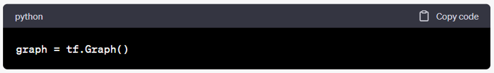
- Create a TensorFlow graph: Create a graph by using TensorFlow's default graph:
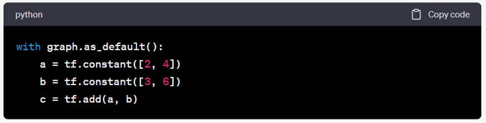
- Define the computational operations: For example, let's define a simple operation that adds two tensors:
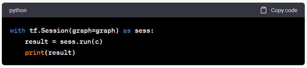
- Run the operations within a session: To execute the operations defined in the graph, open a TensorFlow session and run the session:
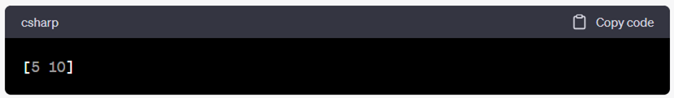
- Run the code: You should see the result printed, which is the element-wise sum of the two tensors:
This simple example demonstrates the basic structure of coding with TensorFlow. You define a computational graph with operations and then run those operations within a session to obtain the results. From here, you can explore more complex operations, build and train neural networks, and work on various machine learning tasks using TensorFlow.
Remember to refer to the official TensorFlow documentation and other learning resources for more advanced coding practices, tutorials, and examples.
Learning Activity
Visit the TensorFlow website and view the learning/support options available:
https://www.tensorflow.org/
Coding activity: coding with TensorFlow to build and train a neural network
Here's an example code that demonstrates a step-by-step process of using TensorFlow to build and train a simple neural network for image classification on the MNIST dataset.
The code shown below can be accessed here.
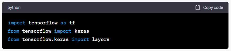
- Import the necessary libraries. TensorFlow and its sub-modules are imported to access the required functions and classes for building the neural network.
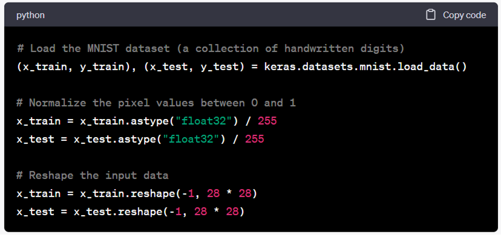
- Load and prepare the dataset. The MNIST dataset, which consists of grayscale images of handwritten digits, is loaded using the keras.datasets.mnist.load_data() function. The pixel values of the images are normalized between 0 and 1, and the input data is reshaped to match the expected input shape of the neural network.
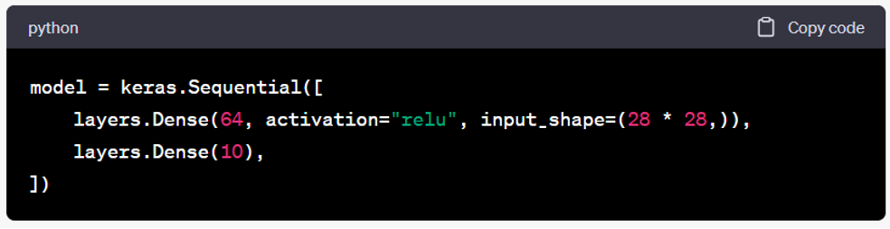
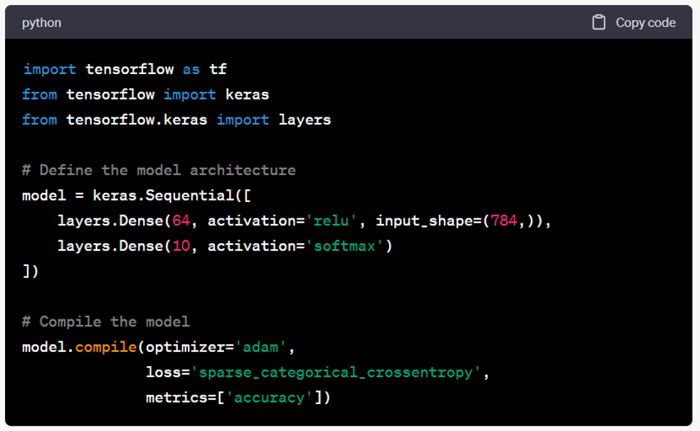
- Define the neural network architecture. A sequential model is created using keras.Sequential(), and two dense layers are added. The first layer has 64 units and uses the ReLU activation function. The second layer has 10 units, representing the number of classes (digits 0-9).
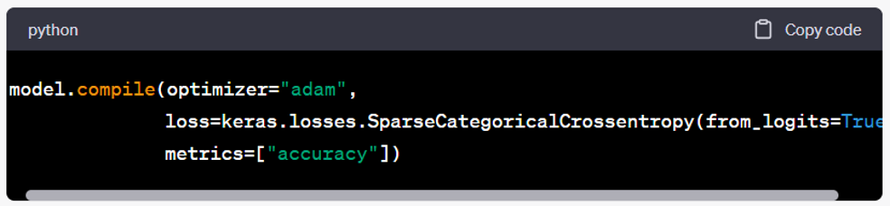
- Compile the model. The model is compiled using the Adam optimizer, sparse categorical cross-entropy loss function, and accuracy as the evaluation metric.
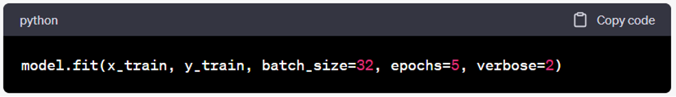
- Train the model. The model is trained using the fit() function, where the training data (x_train and y_train) is passed along with the batch size, number of epochs, and verbosity level.
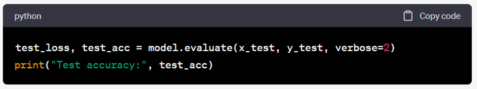
- Evaluate the model. The trained model is evaluated on the test data (x_test and y_test) using the evaluate() function. The test loss and accuracy are calculated and printed.
Keras is a high-level neural networks API written in Python that runs on top of TensorFlow. It provides an easy-to-use interface for building and training deep learning models.
Coding Activity
Here's an example of creating a Keras model using the Sequential API. The code shown below can be accessed here.
- A sequential model is created using keras.Sequential(). The model architecture is defined by adding layers to the sequential model. Here, we have a dense layer with 64 units and ReLU activation as the first layer, and a dense layer with 10 units and softmax activation as the second layer.
- The model is compiled using the compile() method. Here, we specify the optimizer (e.g., Adam), the loss function (e.g., sparse categorical cross-entropy for multi-class classification), and the metrics to evaluate the model's performance (e.g., accuracy).
- Once the model is compiled, it is ready to be trained on the data using the fit() method. This involves providing the training data (input features and corresponding labels), specifying the batch size and number of epochs, and optionally specifying validation data for monitoring the model's performance during training.
The fit() method updates the model's parameters using backpropagation and adjusts them to minimize the specified loss function. The model is trained for the specified number of epochs, with the training data divided into batches of size 32. Validation data can be provided to evaluate the model's performance on unseen data after each epoch.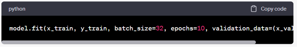
- After training, the model can be used for making predictions on new data using the predict() method. The predict() method takes the input data and returns the model's predictions.
Overall, Keras provides a user-friendly and intuitive way to build, compile, train, and evaluate deep learning models. It abstracts away the complexities of low-level operations, allowing researchers and practitioners to focus on designing and experimenting with various neural network architectures.
Learning Activity
Use information from this course and your own research to consider the following questions:
- What is parameterized learning and what are its benefits and challenges?
- What are the functions of weights and biases?