
With the understanding of the different ways to link your spreadsheet and automate some spreadsheet processes through both programming-based and non-programming-based methods, you can now start processing data into a spreadsheet. A spreadsheet is a useful tool in many business applications such as financial reporting, business analysis and general business accounting, among others. The methods you will learn in this chapter will help you in creating a variety of workplace spreadsheet documents.
Using a spreadsheet involves processes in handling data entries such as entering, checking and amending data. In some cases, you will also need to know how to use data from applications outside Excel and integrate them into your spreadsheet. It is important to learn the different steps in creating and using spreadsheets because it is one of the most widely used document formats in business. You will encounter at least one form of spreadsheet in your day-to-day work. You must know not only how to read through data contained in spreadsheets but also how to input and review data.
In this topic, you will learn how to:
- enter, check and amend data according to organisational and task requirements
- import and export data between compatible spreadsheets and adjust documents, according to software and organisational procedures
- use the help function to overcome problems with spreadsheet design and production
- preview, adjust and prepare spreadsheet in accordance with organisational and task requirements.

When working with spreadsheets, the formulae are only as good as the data entries. Spreadsheets must be populated with data to be able to perform the requirements of the task.
Data entry and checking
There are two ways to enter data into Excel:
- Manual data entry
- Importing data from another source
Manual data entry is done by simply selecting a cell and entering the data you want to put in that cell. Meanwhile, importing data involves using data from a separate file in your spreadsheet.
After entering all the data needed based on your task requirements, the next step is to check and amend the data as needed. Since you are working mostly with numeric values in Excel, it is easy to make errors in calculation. It is important to check and amend the data so that your final spreadsheet output is accurate and consistent with your initial data entries.
Checking Data
Data checking is the process of ensuring the quality and correctness of the data entries in your spreadsheet. Due to the automated nature of spreadsheets, it is very easy for these errors to destroy the quality of your data if unchecked. Remember that your output data quality is only as good as the data entered into your functions and formulae.
There are two methods for checking your data (whether the data has been entered manually or imported):
- Validation
- Verification
Data Validation
Validation is the process of checking the data to ensure that it meets certain requirements, the most important of which is that the data must be valid. Validation generally makes use of the following checks:
- Allowed character check: to ensure that only certain allowed characters are entered in a field
- Field length check: to ensure that the correct number of character have been entered
- Logic check: to ensure that an input will not produce a logical error such as a divide-by-zero error
- Presence check: to ensure that all fields have been populated and do not move on unless they have
- Range check: to ensure that all data falls within an accepted range of values
- Spelling and grammar check: to ensure that there are no spelling or grammatical errors
- Table lookup check: to ensure that the data entered is consistent with data in a valid list of entries which is stored in a database
- Type check: to ensure the correct type of data (numeric, text etc) has been entered into the field
- Uniqueness check: to ensure that the value is unique and has not been entered more than once
Excel can automatically manage much of the data validation process for you. You can use data validation to limit the data that can be entered into a cell. In this process, you are setting a rule for the users of your spreadsheet on what form the data should take.
Alternatively, you can choose to allow users to still input invalid data but give them a warning window when they type the data into a cell. You can also provide instructions to the user on what type of data to enter in a cell and help them resolve errors.
Data validation options can be found in the ‘Data Tools’ group of the Data tab.
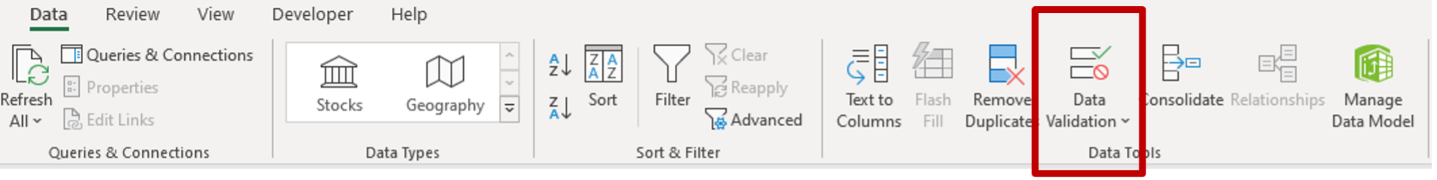
Clicking on this button displays the ‘Data Validation’ dialogue box, which has three tabs:
- Settings
- Input Message
- Error Alert
The ‘Settings’ tab allows you to designate validation criteria to which data must conform in order to be accepted as a valid entry for the cell.
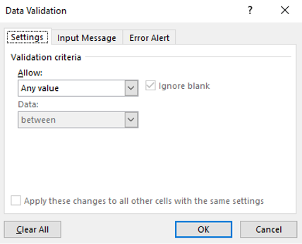
You can set the validation criteria to allow the following:
| Validation Criteria | Description |
|---|---|
| Any value |
|
| Whole number |
|
| Decimal |
|
| List |
|
| Date |
|
| Time |
|
| Text length |
|
| Custom |
|
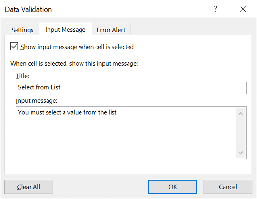
You can use tools in the ‘Input Message’ tab within the Data Validation dialogue box to display a message whenever a user selects a cell.
For example:
The ‘Error Alert’ tab of the Data Validation dialogue box can be used to generate an alert message whenever a user enters invalid data.
For example:
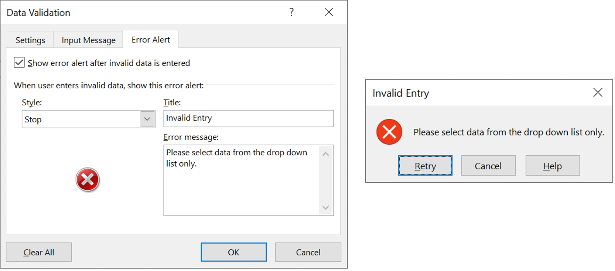
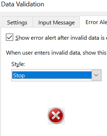
In the drop-down menu, you have three options to choose the style of the error alert. Each style produces a slightly different alert:
Stop
Prevents users from entering invalid data in a cell. Users can click on one of the two options:
- ‘Retry’ – to re-enter valid data
- ‘Cancel’ – to remove the invalid entry
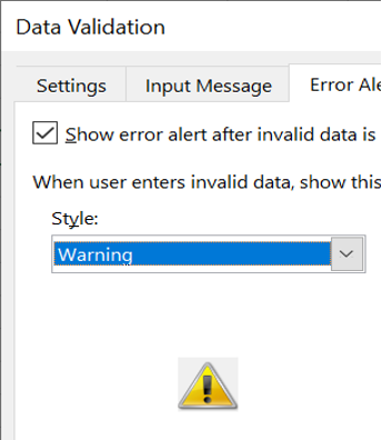
Warning
Will warn users that the data they have entered is invalid without preventing them from entering it.
Users can click on one of the three options:
- ‘Yes’ – to accept the invalid entry
- ‘No’ – to edit the invalid entry
- ‘Cancel’ – to remove the invalid entry
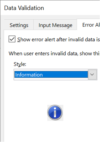
Information
Will inform users that the data they entered is invalid without preventing them from entering it.
Users can click:
- ‘OK’ – to accept the invalid value
- ‘Cancel’ – to reject it.
Data Verification
Data Verification is another method of ensuring data quality. It is the process of checking that the data entered (or imported) is accurate, consistent and reflects the intended purpose. Data verification primarily makes use of the following methods:
- Double entry: where the data is entered twice and each record is compared to the other, if both entries are the same then it is assumed the entry is accurate.
- Proofreading: where the data entered is checked against the data in the original document to identify errors.
It is important to check both your data validity and accuracy to ensure the integrity of your data output. Use data validation to make sure that the data is correct and data verification to make sure that the data is accurate.
Amending Data
Amending data comes hand-in-hand with the checking process. After checking your data using verification and validation procedures, you can now amend the data to address issues identified during the checking stage. This is important because, in a spreadsheet, much of the data you enter is linked to one another. If you do not amend the data errors spotted during checking, your entire workbook and other workbooks may show incorrect data.
Amending data may involve:
- correcting data in source cells
- editing functions and formulae that result in errors.
In Excel, you can amend data by entering ‘Edit’ mode. Excel enters edit mode when you double-click on a cell that already contains data. For reference, you will see the word ‘Edit’ on the bottom left of the application window.
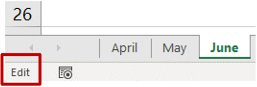
Once you are in ‘Edit’ mode, you may amend the data in the selected cell by typing in the cell directly or by using the formula bar.
When Excel is in ‘Edit’ mode, the functionality of the program is limited to manipulating the values of the selected cell only. This means that you cannot make changes to formatting and layout while you are in ‘Edit’ mode. The movement of your arrow keys will also be limited to the selected cell.
Organisational and Task Requirements for Data Entry, Checking and Amendment
In some cases, your supervisor may require you to enter new data into an existing spreadsheet or template. You may also be asked to review spreadsheets created by others and check them for correctness. When doing these kinds of tasks, it is best to refer to the organisational and task requirements. Some parts of a spreadsheet may contain complex formulae, so entering new data may change multiple cells. If you are unsure which cells to use for your data entries, it is best to consult your supervisor or the original author. This also applies when you check and amend data in a spreadsheet. It is important to collaborate with other personnel involved in creating the spreadsheet and make sure that you all agree with changes to be made.
In addition, data entered in spreadsheets may also be confidential and should reflect in specific documents only. It is important to know your organisation’s privacy and confidentiality procedures to know who is allowed to access your spreadsheet.
Some organisations will also have a specific process in error checking and amendment. This is to ensure a standard in the quality of data reflected in spreadsheets. For example, after checking a spreadsheet you created on your own, you may be required to submit it to someone else for further checking and amendment.
Practice Exercise
Download the following Excel file and the Your IT Pty Ltd practice exercise instructions to complete this exercise.
After you have completed the practice exercise, you can check the sample answer here.

The common process of manually entering data into cells may become tedious when your task involves multiple sets of data from different sources. In the same way, there are times when multiple data entries from your spreadsheet will also be used in other spreadsheets. Excel provides solutions to these through its Importing and Exporting features.
Importing data is the process of automatically entering the data contained in a separate file into your spreadsheet. Doing this will simplify the process of entering large data sets into your spreadsheet. Data to be imported should follow file formats that are compatible with Excel.
Exporting data is the process of saving your spreadsheet in a file format different from its current format (i.e. .xlsx). This is done for ease of import into other programs that may use spreadsheet data.
The primary benefit of data import and export is the convenience of data entry. You would not have to go from cell to cell, manually typing the correct values for each. Additionally, by importing data from a source, you avoid any human error that comes with manual data entry.
While these two processes will save you time in data entry, you still have to take precautionary measures when importing and exporting. Data import and export involves using other files outside your spreadsheet. To avoid data errors or breaches coming from importing and exporting, always remember to refer to and follow your organisation’s policies and procedures on importing and exporting data. These policies and procedures may include:
- how and where to access data files
- valid sources of data to be imported
- reviewing data for accuracy before using it in a spreadsheet
- proper file encryption for exported data
- how to label and store exported data.
Following these organisational policies and procedures will ensure that your data entries are correct, even if some are imported from other files. It will also ensure that all files for import and export are secured in accordance with security and privacy policies.
Importing Data
Aside from manual data entry, the other means of entering data into your spreadsheet is by importing the data from another source. Because many different spreadsheet applications have different file formats, it is often useful to import and export data using simple text documents.
These documents contain what is called raw data with no formatting information. The data entries are separated by a specific character called a ‘delimiter’. Common delimiters used to separate data entries are:
- Comma
- Tab
- Space
To import delimited text data, take the following steps:
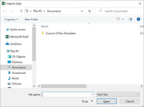
- Go to the ‘Get and Transform Data’ group on the ‘Data’ tab and select ‘From Text/CSV’. This will open the ‘Import Data’ Window.
- Locate and select the text file and click ‘Import’ (initially is the ‘Open’ button but will change to ‘Import’ once you have selected a file). This will open the ‘Navigator Window’ to select the data you want to import.
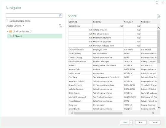
- On the list to the left, select the worksheet of data to import. You will see a preview of the data to the right.
- Click on the ‘Load’ button to import the data into your current workbook. Your selected data will now appear in a new worksheet.
![]()
You can use much the same process to import data from sources other than delimited text files. Excel has the capacity to also import data from the following:
- MS Access
- a webpage
- an SQL server
- an XML file
- a .txt file.
Exporting Data
Data can also be exported from spreadsheet applications using different file formats to allow you to work more effectively with stakeholders using different software applications.
When exporting spreadsheet data using different file formats, use ‘Save As’ rather than the normal save feature in Excel, then select an appropriate file type using the drop-down menu, just like you did for saving as a template.
Useful file formats you can export to include the following:
- .xls – for use in Excel 97-2003
- .txt – for tab-delimited text
- .csv – for comma-delimited text
- .prn – for space-delimited text
- .ods – for OpenDocument Spreadsheet (Open Office Calc)
Adjusting Documents From Data Import and Export
A common problem with importing and exporting data is that the data may not show in the format or layout that you intended. This is because file formats follow different layout parameters.
When you import data from a different file format into Excel, it will appear in a new sheet in your workbook. Your main concern will be to edit the formatting and layout as required and to match similar workbooks. You have a few options to do this:
- Run a formatting macro on the new sheet.
- If you want to edit the formatting of specific cells to match current cells, use the Format Painter tool.
- If the imported data does not follow the format of other documents, manually format the sheet. Remember to record a macro while doing this so that you can apply it to future imported data. You can also choose to save the sheet as a template.
When exporting data from Excel, note that it is possible for the exported file to be used in other spreadsheets. To make the process easier for those who will use your exported data, make sure to:
- organise your data into rows and columns
- limit your entry to one data value per cell
- use and label column and row headers.
Practice Exercise
Open a new Excel workbook and import the sample CSV file below.
Remove the Organisation ID column
Save the file as an Excel workbook with the name 'Top 100 companies.'
Sort the data by:
- the year founded smallest to largest
- the number of employees largest to smallest.
After you have completed the practice exercise, you can check the sample answer here.
Excel is a complex tool that can be intimidating to new users, but if you spend time learning the features of the software, it can make your spreadsheet tasks simpler. However, there will still be times when Excel can get confusing. For example, your functions and formulae may sometimes not work as intended.
Remember that spreadsheet design involves all processes required in preparing a spreadsheet to receive data entries. Common problems that arise when designing spreadsheets are the following:
- incorrect or inconsistent formatting
- unintentional changes to formatting and layout
- incorrect syntax of functions and formulae resulting in errors
- incorrect type of chart/graph used for the selected data
- incorrect application of macros (e.g. steps recorded are incomplete, spreadsheet was not macro-enabled etc.)
- problems with restricting access or protecting a spreadsheet.
Spreadsheet production involves entering data into the spreadsheet and finalising the output. Common problems that arise when producing spreadsheets are the following:
- incorrect data form entered into a cell
- incorrect display of external data sources
- errors resulting from running a macro or formula
- problems with sharing files with other users
- problems with editing files simultaneously with other users
- Excel bugs and freezes.
For these problems and other related problems, Excel offers the Help function to aid you in coming up with solutions.
Excel Help Function
The Excel Help function is a tool you can use to address common problems encountered in Excel. If you are using Excel or a specific Excel feature for the first time, the Help function will provide you with tips to solve your problems or generally improve your workflow.
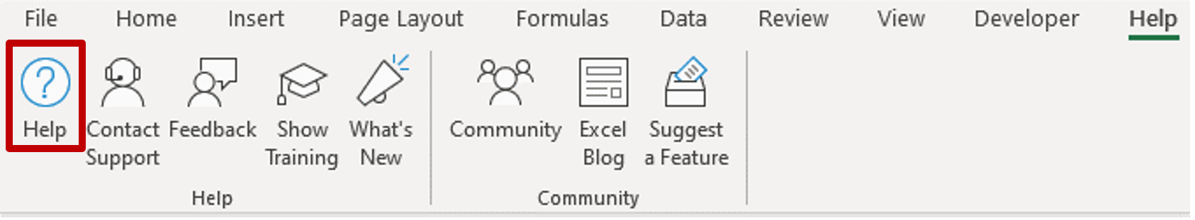
To access the Help function, press [F1] on your keyboard. This will open the Excel Help menu on the right side of your screen. You may also access this by clicking on the ‘Help tab’ and clicking ‘Help’.
The Help function provides important features that you can use if ever you encounter problems while using Excel. These features include:
Help
The ‘Help’ dialogue box will show to the right of the screen, ready for you to type the topic/content of your question.
Contact Support
This allows you to send a question to Microsoft’s online support team.
Show Training
This will take you to online Excel training videos on specific topics. You can search for the subject of the training video by typing in keywords in the search text field.
Community
This will take you to the online Excel Community Hubs to search on a topic and find what others around the world might also be asking. It offers an online community for how-to discussions and sharing best practices in Excel.
Blog Site
This option will take you to the online Excel Blog page to get the latest product announcements and updates.
Resolving Issues with the Help Function
Most of your problems when starting out with Excel can be resolved through the Help function. Note that to access the full capabilities of the Help function, you need to be connected to the internet. Below are the general steps to take to resolve an issue using the Help function. As an example, imagine that you are trying to figure out how to resolve a circular reference in your spreadsheet.
- Press F1 to open the Help menu.
- On the search bar, type your query. In this case, you may type ‘circular reference’. Click the magnifying glass icon beside the search bar or press [Enter] on your keyboard.
- Excel will show you the most common problem related to your query and suggest a solution. If this solution does not address your specific concern, you may view the other results related to your query below the suggested solution.
For some problems, Excel may provide you with links to their online support page.
User Documentation
Some spreadsheet programs will come with a comprehensive user manual or user guide to help you explore the different features of the program. This is a good alternative to the online help function that will be useful if you are not connected to the internet. The manual/guide details the features of the software and how to use each feature. You can use this document to identify the specific software feature you are having issues with and how to resolve these issues.
For Excel, most of the resources are found in the Help function, as discussed above. However, MS Office also published a ‘Quick Start Guide’ to help you with basic problems you may encounter when you start using the program. To use this guide, simply download and open the file and press [Ctrl + F] on your keyboard to access the ‘Search’ bar. You can use this to type keywords related to your problem and locate them in the guide. Some guides may also come with a table of contents for easier navigation.
MS Office also produces downloadable guides that are specific to a common issue you may encounter in Excel. You can access these guides from the MS Office website and search for your topic of concern to find helpful tips that you can apply in your spreadsheets.

The different steps and ways you can preview, adjust, and prepare spreadsheets will be discussed in this section. Excel offers many tools and options that will help you finalise your worksheets. All of these will be useful in making adjustments in formatting, design and layout.
However, it is important to note that these steps will be highly dependent on your organisational and task requirements. As discussed earlier, your formatting, design and layout task requirements answer the question, ‘What should your spreadsheet look like?’. Your organisation may have certain style guides that apply to spreadsheets. They may also have specific policies and procedures that you need to follow when preparing spreadsheets.
It is important to clarify these organisational and task requirements and make the necessary adjustments to your document before you submit your final output. By doing so, you can be sure that the information you entered in your spreadsheet will be read and appreciated by your audience in the way you intended.
Previewing the Spreadsheet
Print Preview
Before printing, it is important to review what the printed pages will look like; this can be done using the ‘Print Preview’ feature.
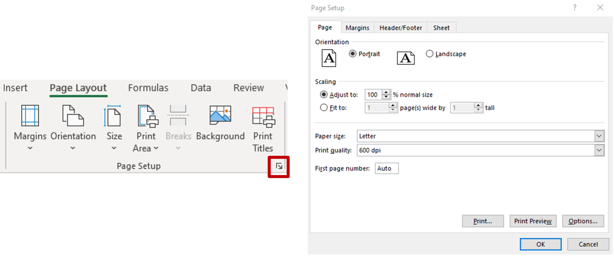
You can access the Print Preview screen by using the [Ctrl] + P keyboard shortcut. This will bring you to the ‘Print’ page, which will show the print preview. Another way is to access the ‘Page Setup’ dialogue box by clicking the small arrow on the bottom right corner of the ‘Page Setup’ group in the ‘Page Layout’ tab. Each tab in this dialogue box will have the ‘Print Preview’ button at the bottom.
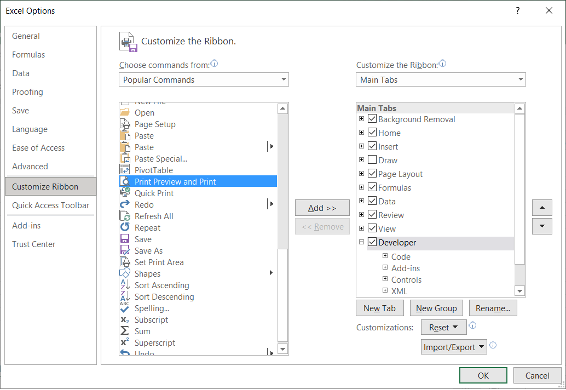
You can also set it up as a custom button on your Quick Access Toolbar by taking the following steps:
- Go to File>Options to open the ‘Excel Options’ dialogue box.
- Click the ‘Customize Ribbon option on the left menu.
- Click ‘Popular Commands’ in the ‘Choose Commands From drop-down list box.
- Scroll down to select ‘Print Preview and Print’ and click the ‘Add’ button.
- Click OK to add the icon to your Quick Access Toolbar.
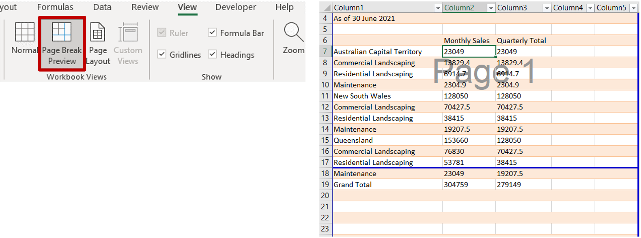
Page Break Preview
The Page Break Preview feature is useful for viewing where the page breaks are in your worksheets. You can access this feature by clicking on the ‘Page Break Preview’ button in the Workbook Views group on the View tab. This is a good way to check if any part of your spreadsheet will be awkwardly cut in between pages when you print or publish. You will be able to quickly adjust the page breaks in your spreadsheet as needed by clicking and dragging the blue border between pages.
Adjusting the Spreadsheet
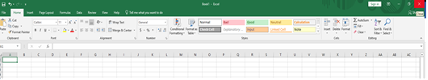
After reviewing your spreadsheet, you now have an idea of what needs to be fixed to make your document more coherent and presentable. Excel offers many options to help you adjust the formatting, layout and design of your spreadsheet. To begin, take a look at the ‘Page Layout’ tab.
Themes
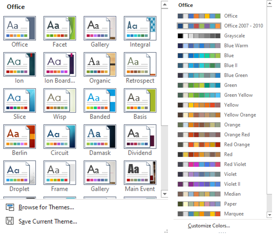
The ‘Themes’ group will give you options on themes, colours, fonts and effects that you can use to make your spreadsheet more aesthetically pleasing and easier to read. You can do this by experimenting with different combinations of colours and fonts. Alternatively, you can also choose from pre-set themes and colour sets offered by Excel.
When adjusting settings under Themes, it is important to take note of any style guides or policies and procedures that your organisation may have in designing spreadsheets. Make sure that the design of your spreadsheet is consistent with the design of other spreadsheets produced by your organisation.
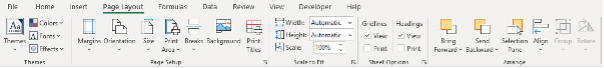
Page Setup
The ‘Page Setup’ group shows buttons for you to adjust the following settings:
- Margins
- Orientation
- Size
- Print Area
- Breaks
- Background
- Print Titles
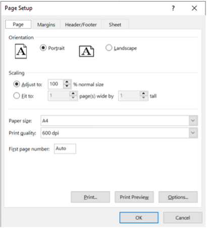
To see and adjust the Page Setup settings in more detail, go to the ‘Page Setup’ dialogue box by clicking on the small arrow at the bottom right corner of the ‘Page Setup’ group. This dialogue box has four tabs: Page, Margins, Header/Footer and Sheet.
The Page tab allows you to set the following:
- Page orientation
- Scaling
- Paper size
- Print quality
- Which page to start printing from
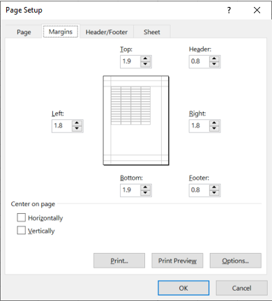
The Margins tab allows you to set and adjust the margins for your worksheets. You have the option of selecting one of three standard margin settings or setting custom margins. This is done on the Margins tab of the Page Setup dialogue box.
When setting custom margins, you can set the following margin options:
- Header margin
- Top margin
- Bottom margin
- Left margin
- Right Margin
- Footer margin
- Centre vertically on the page
- Centre horizontally on the page
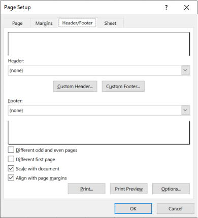
The Header/Footer tab allows you to set and adjust the Headers and Footers for your worksheets.
You also have the option of a different header or footer depending on whether it is an odd or even page.
You can further set your header/footer to scale with the document size and/or choose to align with the page margins or not.
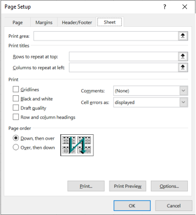
The Sheet tab allows you to set the:
- Print area – the area of the worksheet that you wish to print
- Print titles – the specific rows and columns that you want to be repeated on each printed page
- Appearance of the print-out –enable or disable gridlines, black and white, draft quality, and row and column headings
You also have the option to display comments, notes and errors in your printouts.
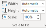
Scale to Fit
The ‘Scale to Fit’ options determine how your spreadsheet will fit into the printed or published pages. By default, your spreadsheet will be set to 100% scale with automatic width and height. You can shrink the width and height of your printout to fit a certain number of pages by clicking on the corresponding drop-down list. Alternatively, you can shrink and enlarge the entire printout by entering a per cent value on the ‘Scale’ field.
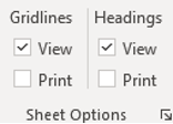
Sheet Options
Under sheet options, you can tick or untick the ‘View’ and ‘Print’ boxes for Gridlines and Headings. The ‘View’ boxes will toggle your current view of gridlines and headings. Meanwhile, the ‘Print’ boxes will toggle whether gridlines and headings will be visible in your printouts.
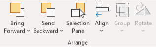
Arrange
The options under the ‘Arrange’ group applies to objects that do not go inside individual cells, such as images, charts and graphs. These settings allow you to organise the arrangement of the different objects in your worksheet in relation to each other.
Preparing the Spreadsheet
So far, you have previewed your spreadsheet and made the necessary adjustments on formatting, layout and design. Your next step is to prepare the spreadsheet for presentation and storing.
Before you proceed with creating graphs and charts, you must ensure that as much as possible, there are no more errors and formatting issues in your spreadsheet. This is important because any errors in the data you entered will also reflect in further reports and presentations that use your spreadsheet as a resource. Formatting issues may also cause confusion in the interpretation of data contained in the spreadsheet.
Preparing the spreadsheet involves going back to your planning document and checking to see if all task requirements have been addressed. Remember that in previous chapters, you have already conducted checks like testing formulae, checking for consistency in design and layout and checking and amending data as needed. Think of preparing the spreadsheet as one final check to see if there are any issues that you missed before.
The following are some guidelines in preparing your spreadsheet for presentation based on task requirements:
| Task Requirements | Guidelines in preparing a spreadsheet for presentation |
|---|---|
| Data requirements | Check if all the given data have been entered and/or integrated into functions and formulae. |
| Linking requirements | Check if cells are properly linked across all worksheets and workbooks. |
| Formatting, design and layout requirements | Check if the spreadsheet followed the organisational style guide and is easy to read and interpret. |
| Functions and formulae requirements | Check if the correct functions and formulae were used in all cells and that no errors and circular references are present. |
| Automation requirements | Check if macros were recorded and applied correctly, i.e. they did not cause any errors to appear in your worksheet. Check also that your spreadsheet is macro-enabled. |
| Import and export requirements | Check that there are no discrepancies between your spreadsheet and other documents connected to it. |
| Organisation requirements | Check for other requirements based on your organisation’s style guide and policies and procedures. |
Once all these requirements have been addressed and finalised, you are now ready to create graphical representations of your spreadsheet data.
Practice Exercise
Download the following Excel file and the Candles 2U practice exercise instructions to complete this exercise.
After you have completed the practice exercise, you can check the sample answer here

Naming, Saving and Storing Spreadsheet
You have so far completed all the steps required in creating your spreadsheet and the presentation materials related to it. One final step you must take is to properly name and store your spreadsheet following organisational requirements.
This is the simplest step in the process, but it is also one of the most critical. Failure to name and store your spreadsheet properly may result in losing your progress or losing your file altogether. Even if you do remember to save your file, if you do not follow the proper naming convention or if you save the file in the wrong folder, your file will be difficult to track and reference.
Naming
Using consistent file naming conventions will help you find spreadsheets quickly and easily. Keeping a consistent file-naming scheme will help ensure that your files remain well-organised, and it will make it easier for you to save several spreadsheets at one time. Follow these recommendations when naming workbooks:
- Be consistent with your naming conventions.
- Write dates in the prescribed format, such as YYYY-MM-DD, for consistency across the organisation.
- Do not use spaces. Use either an underscore or a hyphen but be consistent in which character is used (not both).
- Avoid using special characters (e.g. $,@,%,#,&,*,(,),!,/, etc.) in the file name as they might adversely affect your spreadsheet file.
If your organisation follows certain file naming conventions, be sure to apply those to your document.
Saving and Storing
It is recommended that you save your workbook as early as you can. This is to avoid losing any progress. To save your workbook for the first time, go to File > Save As. Under locations, select ‘Browse’ to open the ‘Save As’ dialogue box. Use this dialogue box to look for your preferred destination folder, then click the ‘Save’ button. Remember to ask and confirm with your organisation the correct folder to use for your document. Also, note if you are required to submit this document via email or cloud storage after you finish it.
When you save your workbook in a non-xlsx file format (e.g. .txt, .csv, etc.), note that some spreadsheet features such as formatting and layout might not be saved. In this case, check the files before using them in other spreadsheets.
Publishing
Publishing is a type of saving you can do on your spreadsheet with the specific purpose of sharing the file to others for viewing. You can set and emphasise what parts of your workbook can be viewed and what will stay hidden. As opposed to a saved spreadsheet, a published spreadsheet cannot be edited by other people unless you, as the author of the document, grant permission. There are three ways to publish a spreadsheet:
- Publish as a PDF file
When you save a spreadsheet as a PDF file, the format, layout, and contents will be locked and cannot be edited. To publish your spreadsheet as a PDF, go to File > Save As and select ‘PDF’ from the file format drop-down list. You can then save the file to your chosen folder or upload it online as required by your organisation. - Publish as Web Page
You can also publish your spreadsheet for the purpose of uploading it on a web server. When you publish your spreadsheet as a web page, the data in the spreadsheet can be viewed but not changed in any way. To publish your spreadsheet as a web page, go to File > Save As and select ‘Web Page’ from the file format drop-down list. You can choose to publish a specific sheet or the entire workbook as a web page. - Publish on the Cloud
You can publish your spreadsheet on the cloud if you want it to be accessed specifically through an online cloud storage drive (e.g. SharePoint, Google Drive, Dropbox etc.). By publishing on the cloud, you can choose who can view and/or edit your document by editing the sharing options provided by your cloud storage service. To publish your spreadsheet on the Cloud, you must save your spreadsheet file on your computer hard drive first. After which, upload the saved file to your cloud storage service. For example, if you upload your file to SharePoint, you can choose the following sharing options shown in the image on the right.
Exiting Application
To exit Excel, ensure that you have saved your work, then click on the red X mark in the top right corner of the application screen. You may also close the application by using the keyboard shortcut, [Alt] + [F4].
If you have more than one workbook opened at a time, you will be closing the active workbook first. By clicking on the close button for the last workbook opened, you will then close the application.
You can also hold down Shift and press the close window button (red x) to close all active workbooks and the application.
Imagine your CBSA manager has asked you to assign contact details against your Aged Debtor spreadsheet so that you can easily contact clients to discuss their outstanding debt. In order to do this, you will need to import information into the following Aged Debtor spreadsheet from the Client Details spreadsheet.
Undertake the following steps to create your macros:
Step 1: Prepare Your Spreadsheets
- Ensure both the Aged Debtor and Client Details spreadsheets are open
- Ensure the Developer tab appears on the ribbon. If not, complete the following steps to select it:
- File
- Options
- Customise Ribbon
- Tick ‘Developer’ box. Click OK. The Developer tab should now appear.
- Ensure the Excel macros are enabled. If they are disabled, the buttons and macros will not work:
- Go to File → Options.
- Select Trust Center → Trust Center Settings.
- Click on Macro Settings and ensure that 'Enable all macros' is selected.
- Click OK and restart Excel if necessary.
Step 2: Create the Macro to Import Contact Details
1. In the Aged Debtor Spreadsheet:
- Go to the View tab on the ribbon.
- Click Macros.
- Select Record Macro and give your macro a name (e.g., FetchContactDetails). Click OK to start recording.
2. Copy Information from the Client Details Spreadsheet:
- Switch to the Client Details spreadsheet.
- Copy the table columns that include Key Contact to Email (including the headings and data).
3. Paste the Information into the Aged Debtor Spreadsheet:
- Switch back to the Aged Debtor spreadsheet.
- Paste the copied data starting in cell H2, which is next to the > 181 column.
4. Stop Recording the Macro:
- Go back to the View tab.
- Click Macros and select Stop Recording.
Step 3: Assign a Button to the Macro
1. Insert a Button:
- Go to the Developer tab on the ribbon.
- Click Insert and select the Button option under Form Controls.
- Click anywhere in the spreadsheet where you want the button to appear (for example, near the contact details).
2. Assign the Macro to the Button:
- When you place the button, it will ask you to assign a macro. Choose the macro you just created (FetchContactDetails).
3. Rename the Button:
- Right-click on the button and select Edit Text or Rename. Name the button Fetch Contact Details.
Step 4: Create a Macro to Clear Contact Details
1. Record a New Macro:
- Go to the View tab and select Macros → Record Macro.
- Name the macro (e.g., ClearContactDetails). Click OK to start recording.
2. Delete the Contact Details:
- Highlight the columns where the contact details were pasted (e.g., starting from H2) and delete them.
3. Stop Recording the Macro:
Go back to the View tab.
Click Macros and choose Stop Recording.
Step 5: Assign a Button to the Clear Macro
1. Insert Another Button:
- Again, go to the Developer tab, click Insert, and select the Button option.
- Place the button in a convenient spot on the spreadsheet.
2. Assign the Macro:
- Assign the ClearContactDetails macro to this new button.
3. Rename the Button:
- Right-click on the button and rename it to Clear Contact Details.
Final Outcome
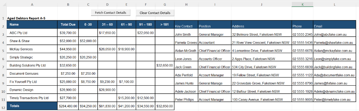
- Now, when you press the Fetch Contact Details button, the relevant contact information will be fetched and displayed next to the Aged Debtors.
- When you press the Clear Contact Details button, the contact details will be deleted, restoring the spreadsheet to its original state.
Learning checkpoint answer
The spreadsheet should look as follows with the buttons:
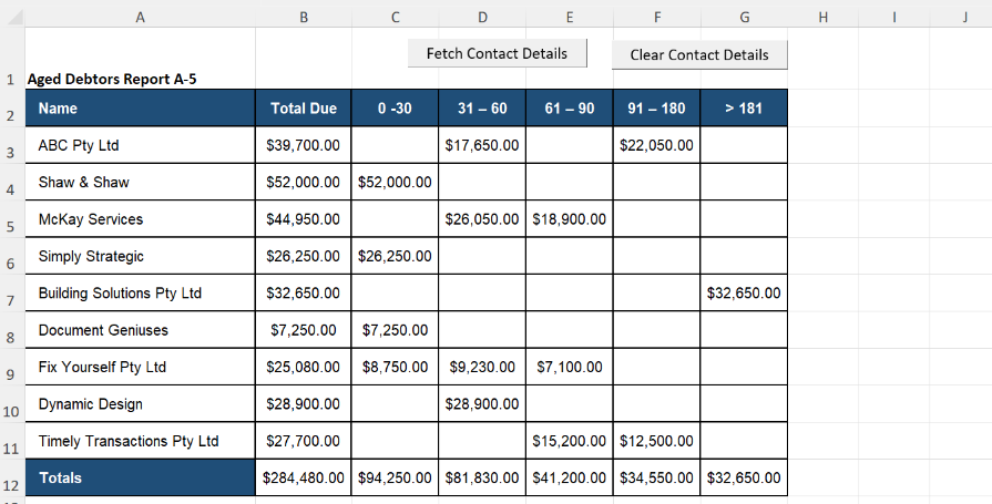
The ‘Fetch Contact Details’ macro should return the following result:
Click here to download a copy of the Aged Deptor spreadsheet with the contact details included.
Note: Although you will be able to see the buttons and the contact details included, the 'Fetch Contact Details' and 'Clear Contact Details' buttons won't work as the macros rely on information from multiple files.
If you need further help with creating macros, watch the following video: