So far, you have set up your work environment and organised your tasks according to the organisational policies and procedures. You have identified the task requirements and what spreadsheet specifications you would need to address these requirements. Specifically, you were able to identify the requirements for the data that you need to reflect in your spreadsheet. At this point, your preparations are complete, and you are now ready to develop a spreadsheet.
In this topic, you will learn how to develop a linked spreadsheet. A linked spreadsheet is a spreadsheet containing data entries that are connected to one another through functions and formulae. These data entries can be linked across cells, spreadsheets and files.
Spreadsheets often contain a large amount of data that are regularly updated. A linked spreadsheet solution will help you connect data entries so that you do not have to manually re-enter and recalculate data.
In this topic, you will learn how to:
- use spreadsheet design software functions and formulae to meet identified requirements
- format cells and use data attributes assigned with cell references according to task requirements
- test formulae to confirm output meets task requirements.
- link spreadsheets according to software procedures
For the purposes of discussion, Microsoft Excel and its features will be used as the reference spreadsheet software for this topic.
Spreadsheet design software formulae
A formula is a mathematical expression that determines the value of a cell. The basic parts of all formulae are:
- Equals sign (=)
- Cell reference
- Operator
The following 4-minute video provides an introduction to using basic mathematical operators and formulas:
Let's take a look
Starting
Equals sign (=) This indicates the start of the formula.
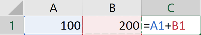
In the example shown above, the formula is entered in cell C1. This means that the final value after entering the formula will also appear in cell C1. In this case, the formula starts with the equals sign (=) followed by the cell reference of the first cell (A1), an operator (+) and the cell reference of the second cell (B1). From this information, you know that the formula in C1 is calculating the result of adding the values in cells A1 and B1.
Once you apply the formula (press Enter), the answer will be shown in C1.
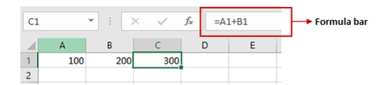
When you select cell C1, you will also notice that the formula you just entered will appear on the formula bar.
Once you apply the formula (press Enter), the answer will be shown in C1.
Cell reference
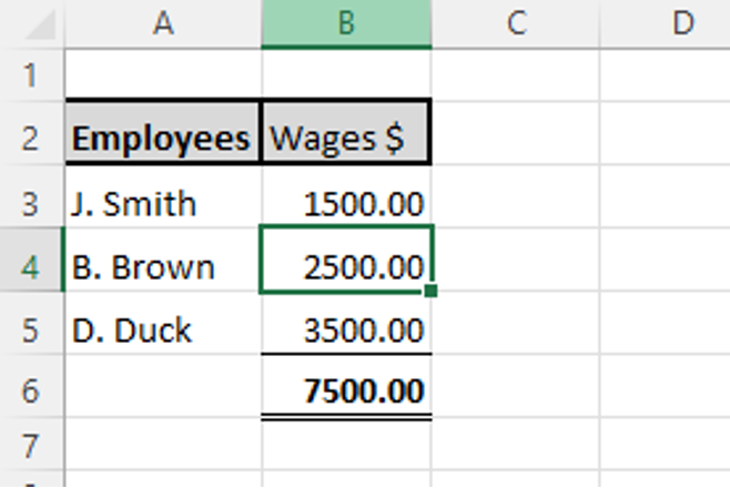
A call reference is a unique label for each cell in a spreadsheet. This is determined by the column letter and the row number. The selected cell in the following example has cell reference B4.
Operators
An operator is a mathematical symbol that dictates the calculation to be performed.
There are different operators that can be used in formulae depending on how you want to relate the values in cells. The four types of operators you can use in Excel:
- Arithmetic Operators
- Logical/Comparison Operators
- Text Concatenation Operator
- Reference Operators
Logical/Comparison Operators are used in Excel to logically compare the two values.
| Operator | Example | What operator does |
|---|---|---|
| = (Equals To) | = A1 = B1 | It compares two values and returns TRUE if both values are equal; If both values are not equal, it returns FALSE. |
| <> (Not Equals To) | = A1 <> B1 | It compares two values and returns TRUE if both values are not equal to each other; If both values are equal to each other, it returns FALSE. |
| > (Greater Than) | = A1 > B1 | It returns TRUE if the value in cell A1 is greater than the value in cell B1; otherwise, it returns FALSE. |
| < (Less Than) | = A1 < B1 | It returns TRUE if the value in cell A1 is lesser than the value in cell B1; otherwise, it returns FALSE. |
| >= (Greater than or equal to) | = A1 >= B1 | It returns TRUE if the value in cell A1 is greater than or equal to the value in cell B1; otherwise, it returns FALSE. |
| <= (Less than or equal to) | = A1 <= B1 | It returns TRUE if the value in cell A1 is less than or equal to the value in cell B1; otherwise, it returns FALSE |
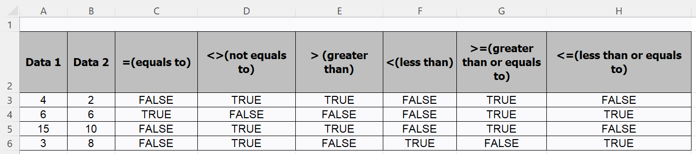
Practice Exercise
Open Excel and use the information below to test your understanding of Logical/Comparison Operators. The first entry has been done for you.
| Data 1 | Data 2 | =(equals to) | <>(not equals to) | > (greater than) | <(less than) | >=(greater than or equals to) | <=(less than or equals to) |
|---|---|---|---|---|---|---|---|
| 4 | 2 | false | true | true | false | true | false |
| 6 | 6 | ||||||
| 15 | 10 | ||||||
| 3 | 8 |
Click here to download a copy of the completed Excel file (where you can see the formulas used).
The Text Concatenation Operator is used to join two or more text strings and produce a single text line.
| Operator | Example | What the operator does |
|---|---|---|
| & (and) | =A1 & B1 | It joins 2 or more strings of text and gets a single text line |
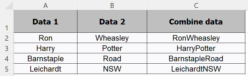
Practice Exercise
Open Excel and use the information below to test your understanding of the Text Concatenation Operator. The first entry has been done for you.
| Data 1 | Data 2 | Combine data |
|---|---|---|
| Ron | Wheasley | RonWeasley |
| Harry | Potter | |
| Barnstaple | Road | |
| Leichardt | NSW |
Click here to download a copy of the completed Excel file (where you can see the formulas used).
Reference Operators are used to refer to a range of cells from the spreadsheet in a formula.
| Operator | Examples | What operator does |
|---|---|---|
| : (colon) | = SUM (A1:B52) | Range operator. Defines the range of cells within the start point and end point reference cells e.g. defines all cells as a range starting from A1 to B52. |
| ,(comma) | = SUM (A1:A8, C5:C22) | Union operator. Combines 2 or more references into a single reference e.g. adds the cell ranges A1 to A8 and C5 to C22. |
| (space) | Insertion operator. It gives reference to cells, which are common in two-range arguments. |
Range Operator
Cell C2 below demonstrates the function of the range operator. It takes a range of all cells starting from A2 to B5 under the SUM function and returns the sum of all 10 values.
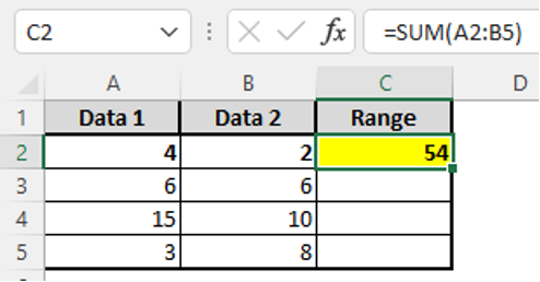
Practice Exercise
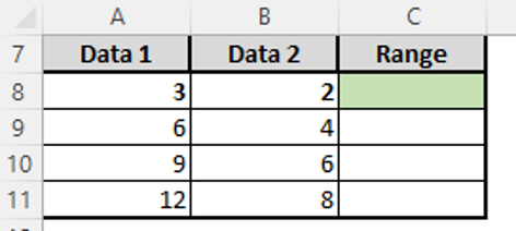
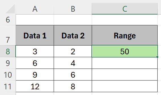
In cell C8, calculate the sum of cells A8 to B11 using the range operator.
Click here to download a copy of the completed Excel file (where you can see the formulas used).
Union Operator
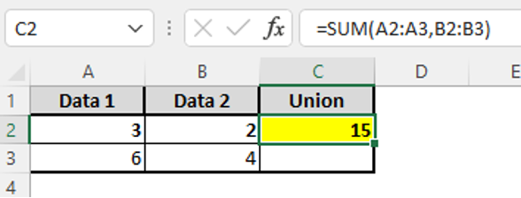
Cell C2 below shows the functioning of the union operator. It takes two ranges as a reference, the first range ( A2: A3) and the second range (B2: B3) under the SUM function. The sum of these two references is given in cell C2.
Practice Exercise
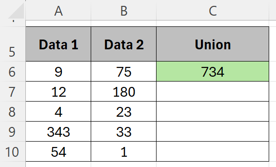
Open Excel and use the information below to test your understanding of the union operator.
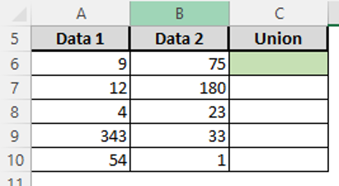
In cell C6, calculate the sum of cells A6 to A10 and B6 to B10 using a union operator.
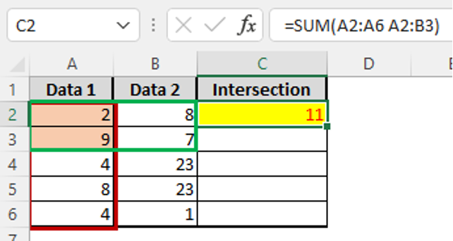
Intersection Operator
Cell C2 below shows the functioning of the intersection operator. It takes two ranges as a reference, the first reference ( A2: A6) and the other as (A2: B3). Using the SUM function, it calculates a sum of values in the cells that are common in both ranges (i.e. cell A2: A3), which is 11.
Practice Exercise
Open Excel and use the information below to test your understanding of an intersection operator.
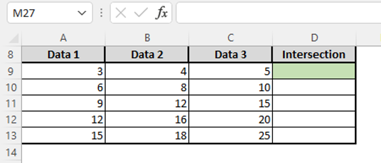
In cell D9, calculate the sum of cells A10 to C11, B9 to B13, B10 to B13 and B10 to C13 using an intersection operator.
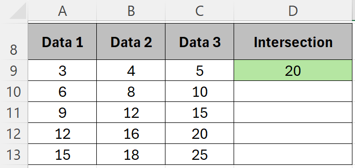
Click here to download a copy of the completed Excel file (where you can see the formulas used).
The following 12-minute video explains and demonstrates how you can use different functions and formulas in Excel.
Tip: If you hover over the video's progress bar, you can see the specific topics covered.
Order of Operations and Operator Precedence
A formula in Excel will always start with the equals sign (=) followed by the operands (numbers and/or cell references) and operators in a specific order. Excel will read and calculate your formula from left to right. However, when you enter multiple operators into a single formula, Excel will solve your formula based on the order of operation priority.
| Operator Priority | Operator |
|---|---|
| 1 | Reference operators (colon, comma, space) |
| 2 | Negation (-) |
| 3 | Percentage (%) |
| 4 | Exponentiation (^) |
| 5 | Multiplication and division (*, /) |
| 6 | Addition and subtraction (+, -) |
| 7 | Concatenation (&) |
| 8 | Comparison (=, <, >, <=, >=, <>) |
The order of operation priority means that Excel will always calculate reference operators first and evaluate comparisons last.
If necessary, you may change the order in which Excel evaluates your formula by using parentheses (). For example, examine the following formula:
= 100 – 8 * 9
Following operator priority, Excel will first multiply 8 and 9, then subtract the product from 100. The cell will display ‘28’ as a result.
= (100 – 8) * 9
However, if you place the operation ‘100 – 8’ inside parentheses, Excel will solve that part of the formula first and then multiply by 9. In this case, the cell will display ‘828’ as a result.
The following 3-minute video explains and demonstrates the basic operator functions, such as addition, subtraction, multiplication and division.
Spreadsheet design software formulae
There is a wide range of formulae that can be used to address spreadsheet problems in Excel. You can combine multiple operators to make complex formulae. However, to make the workflow easier, Excel has predefined commonly used formulae so that they can be accessed faster. These predefined formulae are called functions.
The basic syntax, or structure, of a function is as follows:

- Function name
- Arguments enclosed in parentheses and separated by commas
Every function begins with an equals sign (=) to tell Excel it needs to perform some sort of computation. The function name appears in all capitals and is typically an abbreviation of what the function does. The function name is followed by parentheses, which contain the arguments. Arguments can be numbers or cell references.
By entering arguments, you are instructing Excel to perform your chosen function on those arguments. You can apply a function to multiple arguments or ranges of arguments by enclosing the arguments in parentheses and separating them with commas.
The following are examples of functions commonly used in Excel.
| Function | Description |
|---|---|
| SUM | This function adds all arguments. |
| SUMIF | This function searches for values in a range of cells that meet given specific parameters and then adds them together. |
| SUMIFS | This function searches for values down the first column of a selected range or cells, given multiple parameters. |
| VLOOKUP | This function searches for data in a vertically organised table according to a set of parameters. |
| COUNTIF | This function counts the number of items within a selected range of cells that meet the given parameters. |
| COUNTIFS | This function counts the number of items within a selected range of cells that meet multiple parameters. |
| MAX MIN | This function pulls out the maximum and minimum values from the selected set of data. |
| CONCATENATION | This function combines the contents of selected cells into a new cell. |
| AVERAGE | This function calculates the average of the given arguments. |
| AVERAGEIF | This function calculates the average of all arguments that meet the given criteria within the selected range of cells. |
| STDEV | This function calculates the standard deviation of the given arguments. |
Practice Exercise
Open the Learning Checkpoint Excel Workbook 1 and complete the tabs:
- SUM to test your understanding of the SUM function.
- AVERAGE to test your understanding of the AVERAGE function.
- MAX MIN to test your understanding of the MAX MIN functions.
You can check your answers in the spreadsheet's 'Answers' tab.
The following 19-minute video explains 10 important but more advanced functions that you may find helpful.
Tip: If you hover over the video's progress bar, you can see the specific topics covered.
Once you know how to use functions and formulae, you can use them to address the identified requirements. You can do this by entering your initial data, determining what new data you are required to generate, and using the appropriate functions and formulae to arrive at the required data.
Using formulae and functions to address task requirements
Part of your planning and organisation process was to identify the requirements for your spreadsheet task. You may recall that one of the requirements that you must address involves determining the formulae and functions you need for your spreadsheet task.

Using formulae to address task requirements
Formulae can be used to calculate values and generate new data based on task requirements. Formulae are best applied for quick and simple operations that do not require complex calculations. Earlier, you learned about the different types of operators that you can use in Excel – arithmetic, text concatenation, comparison and reference operators. By using these operators, you can use formulae to address task requirements.

Take a look at the following examples of how to use formulae for different task requirements.
Arithmetic Operators
You can use arithmetic operators to perform basic mathematical operations on cell values.
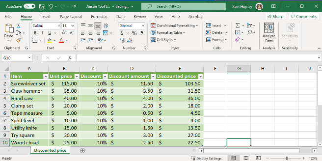
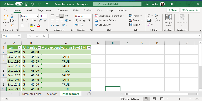
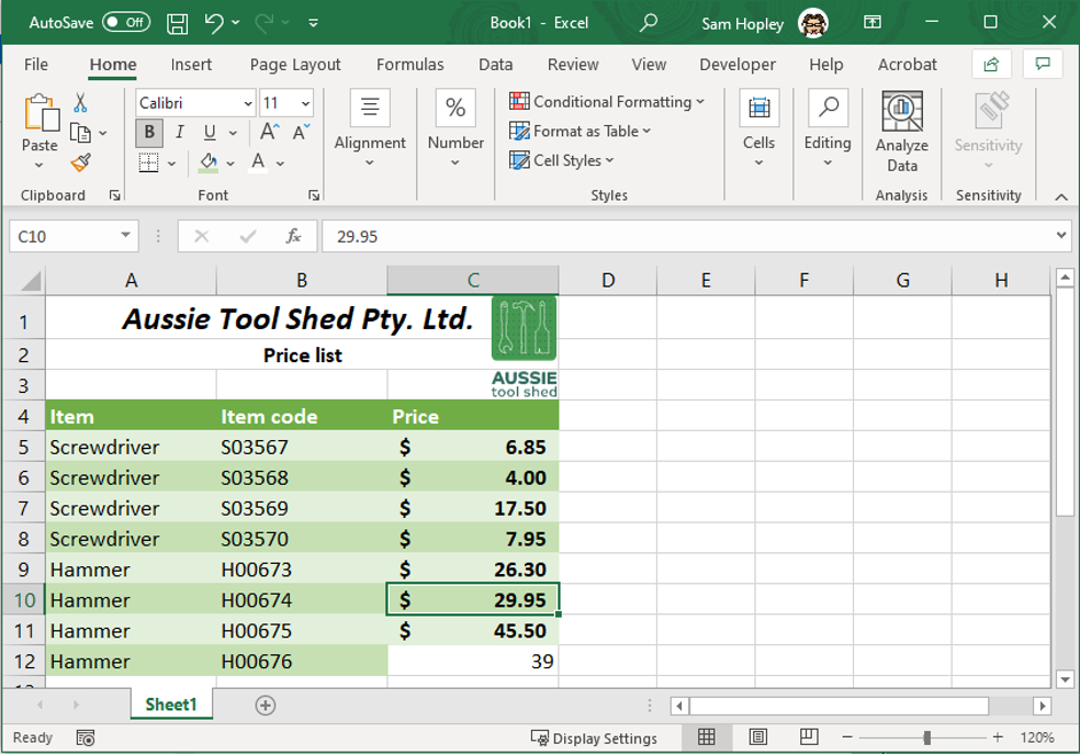
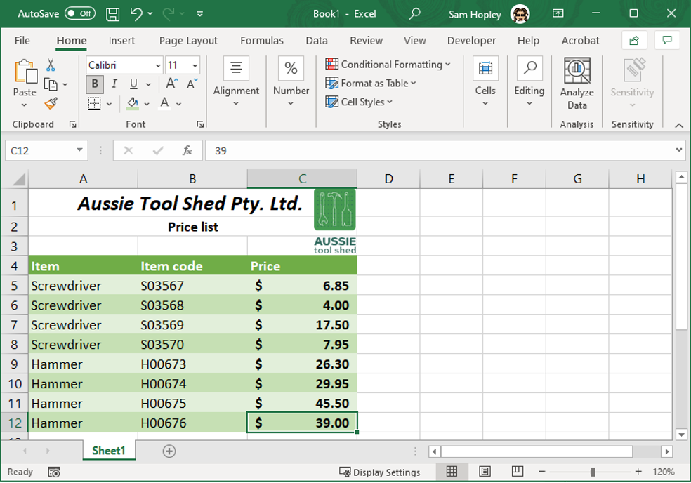
For example, imagine that Aussie Tool Shed is giving a 10% discount on carpentry tools for a limited time. Your supervisor asks you to calculate the discounted prices for each item. The initial data are as follows:
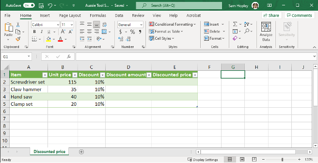
Tip: You can format the values in the discount column as percentages or as decimals. Simply use the drop-down menu in the ‘Number’ category on the ‘Home’ ribbon.
From here, you can use formulae to determine the discount amount and the final discounted price for each item.
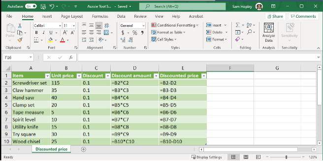
The formulae in column D calculate the discount amounts by multiplying the unit prices in column B by 10% or 0.1, as indicated in column C. The formulae in column E calculate the final discounted prices by deducting the discount amounts in column D from the regular unit prices in column B.
Tip: You can format the values in columns B, D and E as currency. Simply select the ‘$’ symbol in the ‘Number’ format category on the ‘Home’ ribbon.
Text Concatenation Operator
The text concatenation operator is used to connect strings of values into a single line of text.
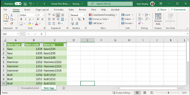
For example, suppose your supervisor at Aussie Tool Shed asked you to combine the item name with the item code to form unique tags for each item. You can do this by using the text concatenation operator in a formula as follows:
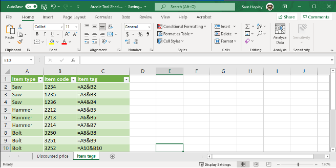
In this case, the final tags were determined by concatenating the ‘item type’ values in column A and the ‘item code’ values in column B.
Comparison Operators
You can use a comparison operator to determine whether a given comparison is true or false.
For example, if you want to determine what items in an inventory are more expensive compared to a selected item, you can do so by using a ‘greater than’ (>) comparison operator. If the item you want to use for comparison is ‘Saw1234’, your formulae will be as shown in the following image:
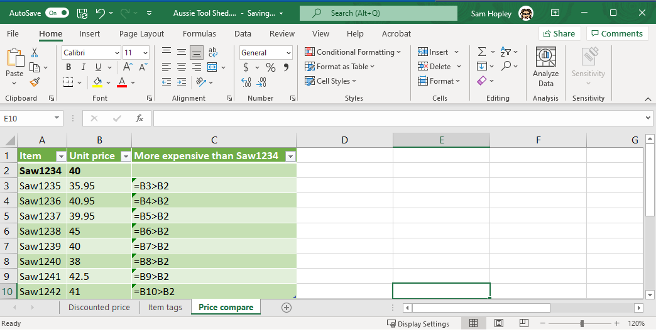
Tip: In this example, the cell reference for the comparison item (B2) remains the same in every row. Excel can autofill formulae in some situations. To make sure the reference cell remains the same, add a ‘$’ symbol in front of the column letter and in front of the row number. For example, the formula in C3 becomes:
=B3>$B$2’
Reference operators
Reference operators are used to easily group a range of cells and perform formulae and functions on them.
For example, if you needed to calculate the total of a purchase order, you could write a formula using addition symbols (+). You can perform the same task using the SUM function.
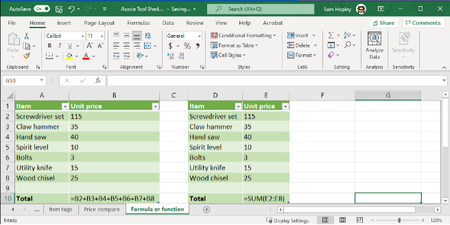
In the previous image, the table on the left shows the addition formula where each cell reference from A2 to A8 is listed. The SUM function, shown in the table on the right, uses the colon reference operator (:) to indicate the range of cells from A2 to A8.
Tip: Excel will automatically create a reference operator if you click and drag to highlight a range of cells.
Using functions to address task requirements
Functions are likely to be quicker than formulae when you need to perform more complex calculations with and manipulation of the data. In Excel, the functions are grouped into categories so that you can easily identify the most appropriate function for the task. You can access these categories and their functions by going to the ‘Function Library’ group under the ‘Formulas’ tab.
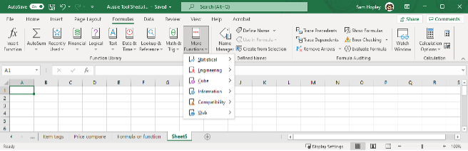
Excel has the following categories in the function library:
- Compatibility
- Cube
- Date and time
- Engineering
- Financial
- Information
- Logical
- Lookup and reference
- Math and trigonometry
- Statistical
- Text
- Web.
However, for the business application of Excel, you will most likely require functions with the following categories:
- Date and time
- Financial
- Logical
- Lookup and reference
- Math and trigonometry
- Statistical
- Text.
The following 12-minute video explains new Excel functions, such as dynamic sorting and data filtering, discovering unique values, enhanced lookups and numerical sequences.
Let us look at each of these seven categories in more detail.
For each function mentioned, the general syntax will be outlined. The syntax is the information you need to put into the function for the computing to occur correctly. To add the information, either enter the raw data or enter the cell reference for the cell containing the relevant data for each argument.
Excel displays the syntax for each formula when it is selected. You do not need to remember them all!
Date and time functions
You can perform various calculations involving dates and times and reflect these in your Excel spreadsheet by using date and time functions. In business, these functions will be useful in marking your documents with the date and time as well as in computing targets and deadlines.
The following table provides an overview of some different date and time functions.
| Function | Description | Syntax |
|---|---|---|
| DATE | Enters the specified date in the specified format. | =DATE(year,month,day) |
| NOW | Enters the current date and time, which automatically updates. | =NOW() Note: This function has no arguments, but the parentheses must be included. |
| TIME | Enters the specified time in the specified format | =TIME(hour,minute,second) |
| TODAY | Enters the current date, which automatically updates. | =TODAY() Note: This function has no arguments, but the parentheses must be included. |
| NETWORKDAYS | Calculates the number of whole workdays between the specified dates. | =NETWORKDAYS(start_date, end_date,holidays) |
The following 3-minute video tutorial demonstrates how to add the current date and time to a spreadsheet.
For example, some documents require you to input the date of the last edit made. Manually typing in the date every time you edit the document is prone to error. There may be times when you forget to edit the date or type the wrong date by mistake.
To avoid this, you can use the TODAY function to generate the current date. Every time the spreadsheet is edited, the cell containing the TODAY function will automatically update with the current date.
Financial functions
Excel includes a broad range of financial functions, which are useful for performing financial analyses such as determining the following:
- Interest rates
- Current values of investment
- Future values of investments
- Term durations for loans and investments
- Impact of increasing/decreasing payments on a loan.
For example, for computing payments on a loan, the following functions will be useful:
| Function | Description | Syntax |
|---|---|---|
| IPMT | Calculates the interest payment due for a given period. | =IPMT(rate,per,nper,pv,fv,type) |
| NPER | Calculates the number of payment periods needed to pay off a loan. | =NPER(rate, pmt, pv, fv, type) |
| PMT | Calculates the periodic payment for a loan over the life of the loan. | =PMT(rate,nper,pv,fv,type) |
| PPMT | Calculates the principal payment due for a given period. | =PPMT(rate,per,nper,pv,fv,type) |
| RATE | Calculates the interest rate per period. | =RATE(nper,pmt,pv,fv,type,guess) |
To use the functions above, you need to define and input the following information into the function as required by the specific syntax:
- rate – the interest rate for the given period
- per – the period used to compute payment
- nper – the total number of payment periods
- pv – the present value of the projected payments
- fv – the future value after all payments have been completed
- type – this indicates when payments are due with either a '0' (due at the end of the period) or '1' (due at the beginning of the period)
- guess – your own projection of what the rate will be.
Each function will specify the arguments it requires in the syntax. Simply select or enter the appropriate cell reference to add the information to the function.
For example, suppose you want to compute the interest payment on a loan due for a given month. You have the following data:
- Loan amount = $10,000.00
- Interest rate = 5%
- Total number of payment periods = 60
- Payment periods per year = 12
In this case, you need to use the IPMT function to return the interest payment due for the month. The correct IPMT function arguments are shown in the following image.
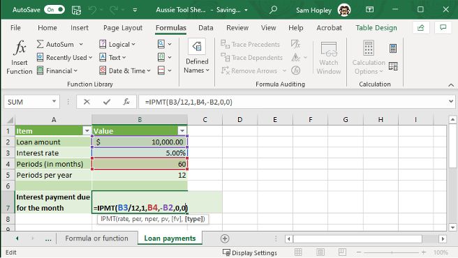
Tip: When you click inside a formula or function, the arguments and cells are colour-coded so you can easily see where each value comes from.
The following 8-minute video tutorial explains the above-outlined finance functions:
Logical functions
Excel includes several logical functions that use comparison operators to introduce decision-making processes to your spreadsheets. Logical functions return either a TRUE or FALSE result after evaluation. For instance, the IF function analyses a cell or range of cells and determines whether the values meet a given condition. The function produces one output when the value is TRUE (meets the condition) and a different output for a FALSE (does not meet the condition) result.
The following table outlines some common logical functions.
| Function | Description | Syntax |
|---|---|---|
| AMD | Enters the word TRUE, if all enclosed arguments are true. | =AND(logical1, [logical2], ...) |
| FALSE | Adds the word FALSE to the cell. | =FALSE( ) Note: This function has no arguments, but the parentheses must be included. |
| IF | Enters a chosen value if the specified logical test is true and a different value if it is false. | =IF(logical, value_if_true, [value_if_false]) |
| IFERROR | Enters a specified value when the entered formula results in an error. | =IFERROR(value,value_if_error) |
| NOT | Reverses the logic of the argument and enters TRUE when the result is false and FALSE when the result is true. | =NOT(logical) |
| OR | Enters the word TRUE if any of the selected arguments are true. | =OR(logical1,logical2,...) |
| TRUE | Adds the word TRUE to the cell. | =TRUE( ) Note: This function has no arguments, but the parentheses must be included. |
Imagine you are tasked to make an expense report for Aussie Tool Shed. One of the spreadsheet tasks is to determine whether each item in the report stayed within the allocated budget. To show this in your spreadsheet, you can use the IF function, as shown in the following image.
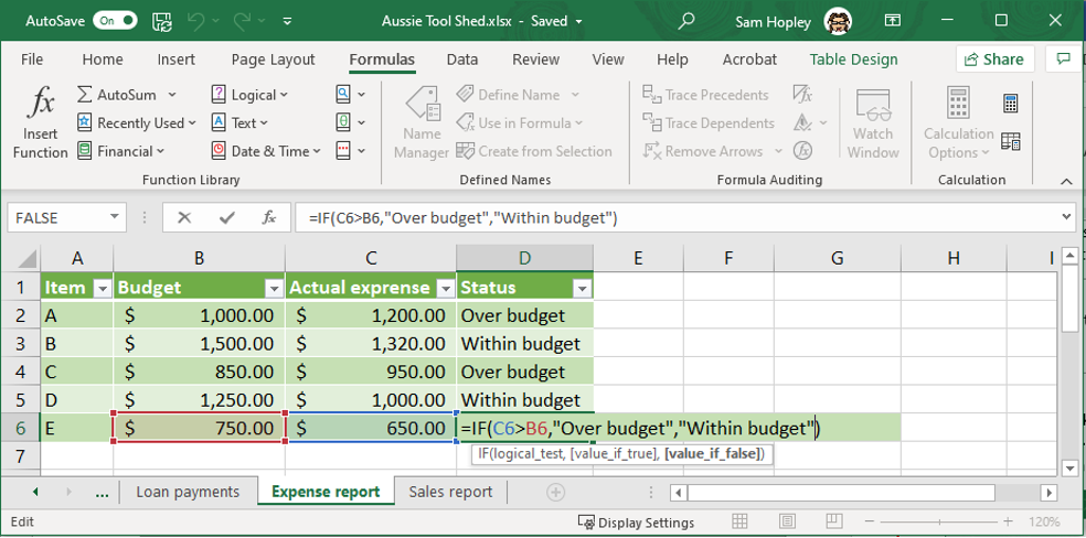
In this instance, the function asks whether the value in column C is larger than that in column B. If the condition is true, the status is set to ‘Over budget’. Where the situation is false, the status is set to ‘Within budget’.
Math and trigonometry functions
Math and trigonometry functions perform common mathematical calculations, including basic arithmetic and trigonometric calculations. Excel also provides functions for working with numerical values, such as rounding or truncating, identifying the sign and generating random numbers.
Some common mathematical functions are described in the following table.
| Function | Description | Syntax |
|---|---|---|
| ABS | Displays the absolute value of a number. In other words, it converts negative numbers to positive numbers and keeps positive numbers the same. | =ABS(number) |
| INT | Removes all decimal places from a value to create a whole number (integer). | =INT(number) |
| PI | Enters the value of pi. | =PI() Note: This function has no arguments, but the parentheses must be included. |
| POWER | Calculates the result of one number raised to the power of a second number. | =POWER(number,power) |
| RAND | Displays a random number between 0 and 1 | =RAND() Note: This function has no arguments, but the parentheses must be included. |
| ROUND | Rounds a decimal value to the number of decimal places you specify. | =ROUND(number, num_digits) |
| SIGN | Displays ‘1’ for positive numbers or ‘-1’ for negative numbers. | =SIGN(number) |
| SUM | Adds the selected cells. | =SUM(number1, [number2], [number3], [number4], ...) |
| SUMIF | Adds the cells only if they meet a given condition. | =SUMIF(range, criteria, [sum_range]) |
| TRUNC | Will retain a specified number of decimal places while removing all others without rounding. Note: If you don’t specify a number of decimal places, TRUNC and INT function in the same way. |
=TRUNC(number,num_digits) |
The following 3-minute video tutorial explains how to use trig (or trigonometry) functions in an Excel spreadsheet:
An example of using mathematical functions would be if you were asked to determine the most profitable business customer of Aussie Tool Shed. In this case, you could use the SUMIF function to only add the sales from specific businesses.
The image below shows the SUMIF function in action.
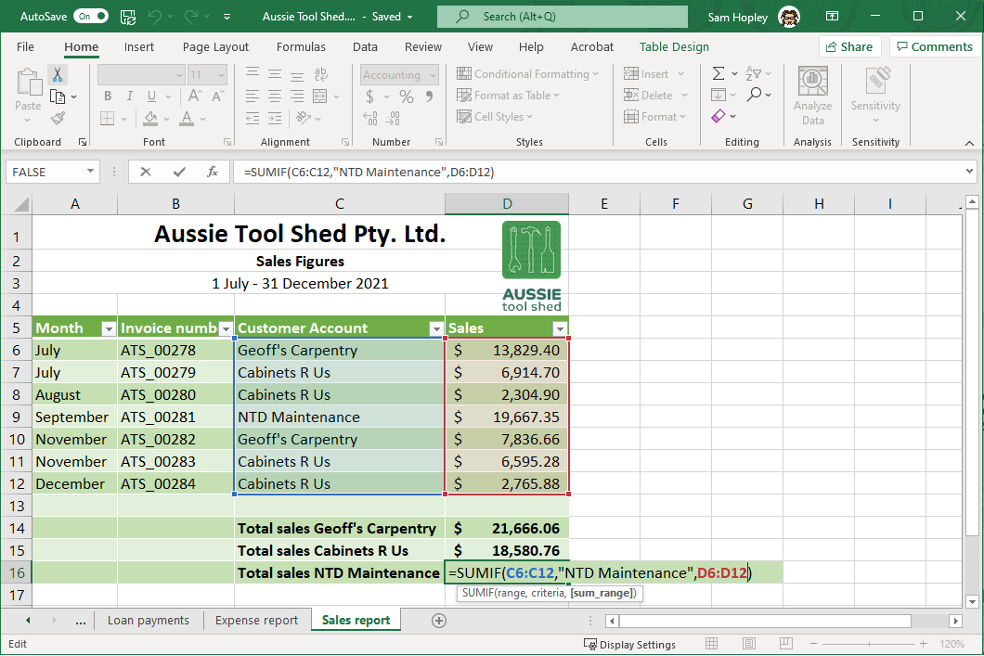
As stated by the syntax of the function, Excel will first check the range, ‘C6:C12’ for the value, ‘NTD Maintenance’. After that, it will calculate the sum of the corresponding values in column D.
Statistical functions
Excel has many statistical functions that can be used to analyse data in a variety of different ways. These functions can be used to find the average value or rank data in ascending or descending order, as well as more complex operations, such as determining the standard deviation.
Some of the more common statistical functions are presented in the following table.
| Function | Description | Syntax |
|---|---|---|
| AVERAGE | Calculates the average of its arguments. | =AVERAGE(number1, [number2],...) |
| COUNT | Enters the number of numerical values in the given range of arguments – it doesn’t count empty cells or those containing text. | =COUNT(value1, [value2],...) |
| COUNTA | Enters the number of cells that contain values in the given range – it doesn’t count empty cells. | =COUNTA(value1, [value2], ...) |
| MAX | Identifies the highest numerical value in the given range of arguments. | =MAX(number1,number2,...) |
| MIN | Identifies the lowest numerical value in the given range of arguments. | =MIN(number1,number2,...) |
| STDEV | Calculates the standard deviation of the range of arguments. | =STDEV(number1,number2,...) |
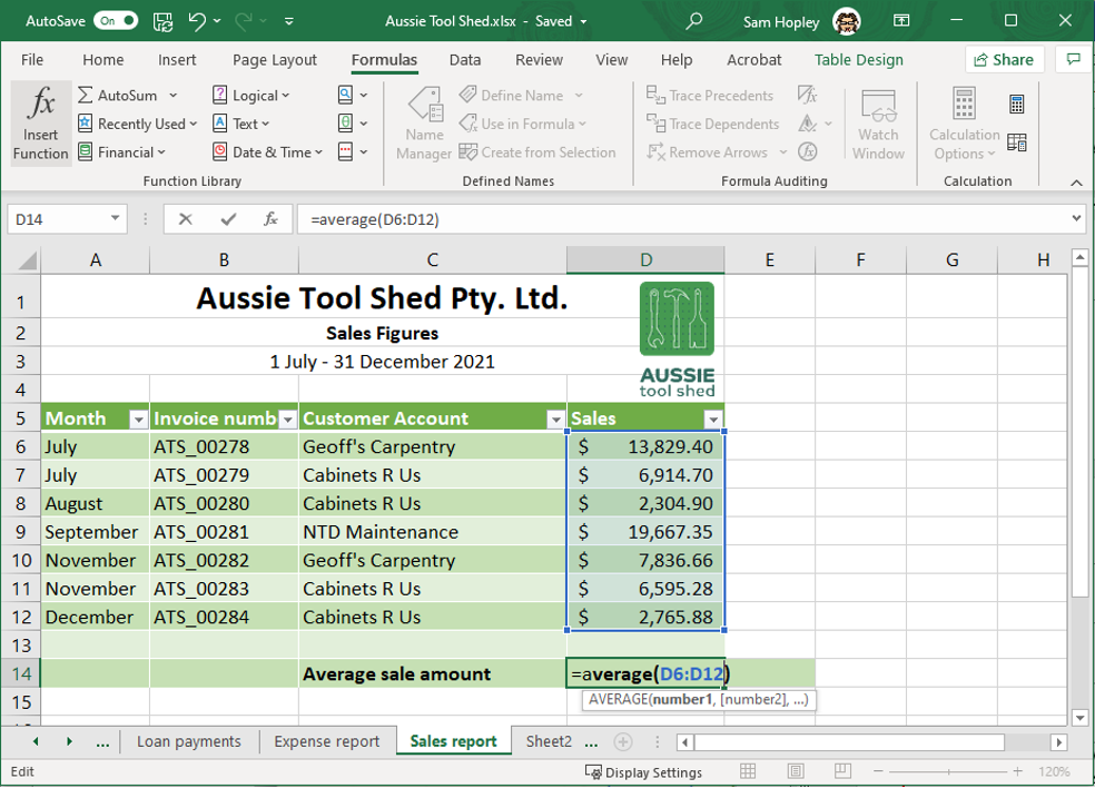
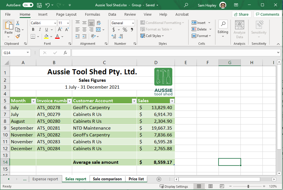
For example, if you were to compute the average sale amount for business customers, you can use the AVERAGE function, as shown in the following image. In this example, the function will compute the average of the values in the selected range, cells D6 to D12.
The following 7-minute video explains statistical functions in Excel, such as average, maximum and minimum, count, conditional count and standard deviation.
Text functions
Excel has useful functions to assist you with working with and manipulating strings of text-based data. Many of these text functions allow you to extract, insert and join parts of the text entry within a cell.
| Function | Description | Syntax |
|---|---|---|
| CONCATENATE | Joins multiple selected cell contents into one text item. Cells must be referenced separately rather than entered as a range. | =CONCATENATE(text1, [text2], ...) |
| FIND | Identifies the location of one text value within another (case-sensitive). | =FIND(find_text,within_text,start_num) |
| LEFT | Identifies the leftmost value based on the specified text and number of characters that need to be identified. | =LEFT(text,num_chars) |
| LEN | Counts the number of characters contained in the specified cell, including spaces in text. | =LEN(text) |
| MID | Identifies specific characters contained within a specified cell, given the specified start position and number of characters required. | =MID(text,start_num,num_chars) |
| RIGHT | Identifies the rightmost value based on the specified text and number of characters that need to be identified. | =RIGHT(text,num_chars) |
| TEXT | Converts a numerical value into a specified text format, as indicated in double quotation marks. | =TEXT(value, format_text) |
For example, suppose your supervisor asks you to compile the first names and surnames of Aussie Tool Shed employees into a single column. You can use the CONCATENATE function, as shown in cell C2 in the following image.
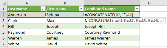
Tip: Include a space within double-quotation marks (“ “) within the function to add a space between cell values.
Lookup and reference functions
Lookup and reference functions help you work with arrays of data. A data array is an organised collection of data of the same type. In Excel, arrays usually take the form of a table. Lookup and reference functions allow you to identify the location of a particular value or to find a value given the location in the array.
You could use a series of logical functions to perform similar tasks. However, lookup and reference functions can greatly simplify the process of finding specific entries within a large data table.
| Function | Description | Syntax |
|---|---|---|
| CHOOSE | Identifies a value from a predetermined list, given the required position in the list. | =CHOOSE(index_num,value1,value2,...) |
| LOOKUP | Searches a column or row to find a specified value from the same position in another column or row. | =CHOOSE(index_num,value1,value2,...)=LOOKUP(lookup_value, lookup_vector, result_vector) or =LOOKUP(lookup_value, array) |
| ROWS | Identifies the number of rows in a selected data array. | =ROWS(array) |
| VLOOKUP | Searches for data in a vertically organised table according to a set of parameters | =VLOOKUP(lookup_value, table_array, col_index_num, [range_lookup]) |
To use the functions above, you need to define and input the following into the function as required by the specific syntax:
- lookup_value – the value you want Excel to look for.
- table_array – the table reference from which the value will be retrieved – typically a range of cells.
- col_index_num – the column reference from which the value will be retrieved, where the left-hand column of the selected range is 1.
- range_lookup – returns whether the match found is ‘TRUE’ (approximate match) or ‘FALSE’ (exact match)
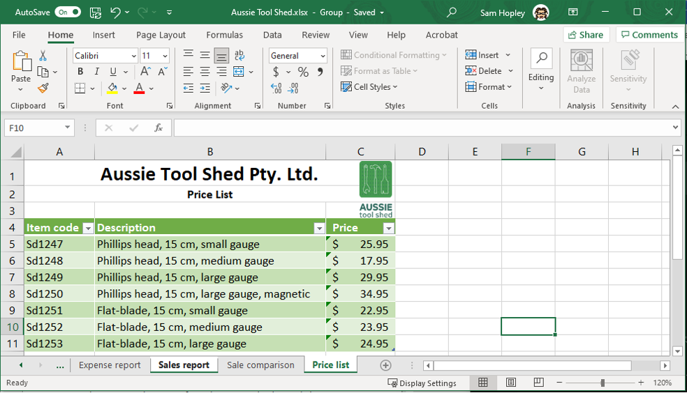
For example, suppose you want to know the price of a particular item from a given price list. You can use the VLOOKUP function as follows:
=VLOOKUP(A13, A5:C11, 3, FALSE)
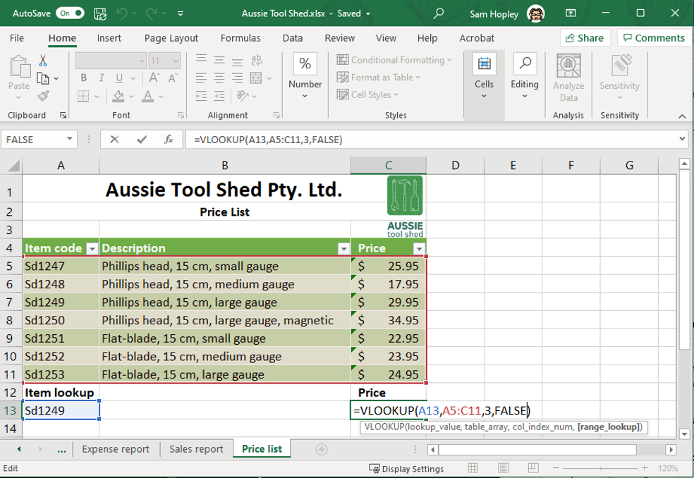
In this example, the lookup_value was given as a cell reference, which means you could change the item code in that cell and find the correct price for that item.
As determined by the syntax:
- Excel searches for the lookup_value in the indicated table (A5:C11)
- Cross-references the located value with the column that contains the required information (in this case, prices in column 3)
- Returns the exact unit price that is in the same row as the located value.
Nested functions
You can combine different functions and formulae. Using one function as an argument for a different function or formula is called nesting functions.
Nesting functions give you the ability to implement complex decision-making and computation processes in a single cell. Keep in mind, however, that as the level of nesting increases, so does the complexity of your formula. A complex formula with multiple levels of nesting can be quite difficult to understand if you need to come back to it later to make a change.
For example, there is a concern that a major business customer is less satisfied with Aussie Tool Shed than they have been in the past. Your supervisor asks you to compare the average monthly sales to this business customer over the last six months with the previous six months to see if there has been any significant change.
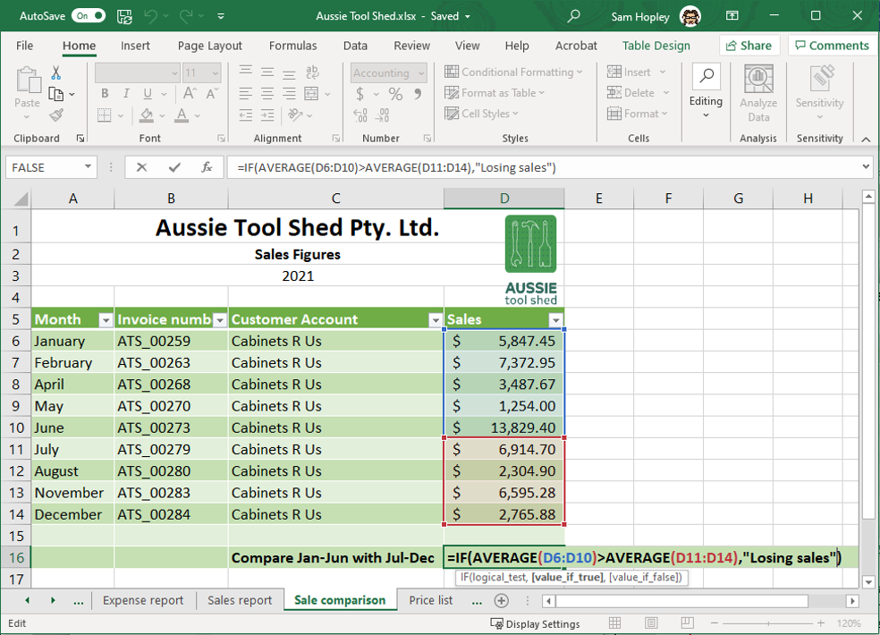
As shown in the previous image, the AVERAGE function is nested twice within the IF function.
=IF(AVERAGE(D6:D14)>AVERAGE(D11:D14),” Losing sales”)
The syntax instructs Excel to calculate the average sales for the two periods and compare them. If the average monthly sales are higher for the first six months than for the second six months, then Excel will enter the phrase ‘Losing sales’.
Practice Exercise
Open the Learning Checkpoint Excel Workbook 1 and complete the tabs:
4. VLOOKUP to test your understanding of searching for data in a vertically organised table according to a set of parameters
5. FIND to identify the location of one text value within another.

When developing spreadsheets, you will often find yourself using the same data across multiple tasks and even across different projects. In these situations, you could duplicate the required data into each spreadsheet. However, copying data can be very time-consuming and increases the chances of errors occurring. Instead, it can be valuable to link the spreadsheets together using the tools provided in your spreadsheet software.
To link spreadsheets, you need to follow the linking procedures specific to the spreadsheet software you are using. This subtopic will discuss how worksheets and workbooks are linked using the software procedures of Excel. Note that other spreadsheet software may follow different procedures for linking. However, all spreadsheet software will have features that allow users to create a linked spreadsheet solution.
The following 4-minute video tutorial explains working with multiple worksheets.
Worksheets and workbooks
Excel allows you to connect your data by linking worksheets and workbooks.
A worksheet is the workspace where you enter data composed of columns and rows of cells. The default worksheet in Excel is labelled ‘Sheet1’ on a tab at the bottom of the window.
You can add a new sheet by clicking the ‘+’ button. Each new worksheet you add will be automatically labelled as ‘Sheet2’, ‘Sheet3’, and so on.
![]()
Where you have multiple worksheets in the same spreadsheet, it is best practice to rename the worksheets to make it easier to find the data you want. To rename a sheet, ‘right-click’ on the sheet name and select ‘Rename’.
A workbook is an Excel file containing one or more worksheets. The filename of a default workbook is ‘Book1’. New workbooks that you will open following the first workbook would be labelled as ‘Book2’, ‘Book3’, and so on. You can rename your workbook to reflect the project or task it services by clicking ‘Save As’ in the ‘File’ menu.
![]()
Linking worksheets
In Excel, it is easy to create, format and edit multiple worksheets at the same time. First, you need to select the worksheets you wish to work with. There are a number of options for selecting multiple worksheets.
- To select a continuous range of worksheets, ‘left-click’ on the first worksheet tab, then hold down the [Shift] key and ‘left-click’ on the last worksheet tab in the selection. This will highlight both tabs selected, as well as all the tabs in between.
- To select specific worksheets that are not in sequence, hold down the [Ctrl] key and ‘left-click’ each worksheet tab you wish to include in your selection.
- To deselect specific worksheets that are currently selected, hold down the [Ctrl] key and ‘left-click’ the worksheet tabs you wish to deselect.
Once you have selected multiple worksheets, any formatting changes, data or formulae you enter into one of the selected worksheets will be entered into all the other selected worksheets at the same time.
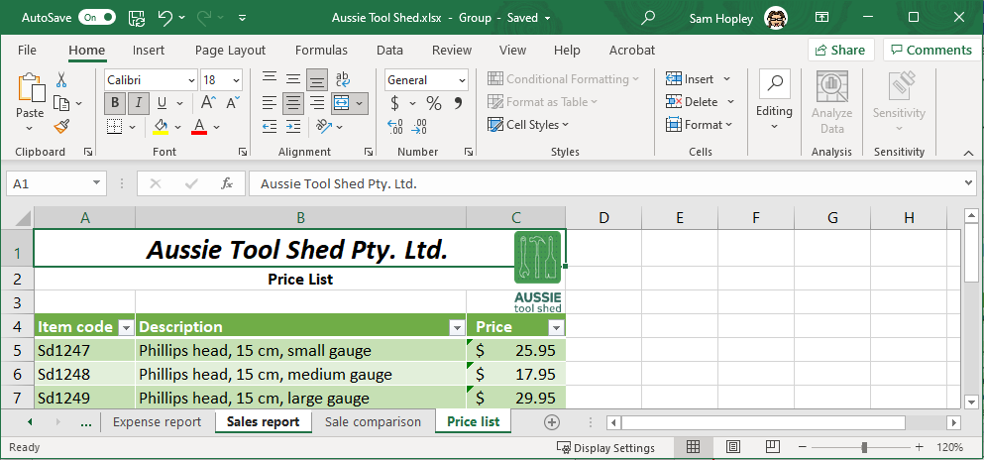
For example, if you want ‘Aussie Tool Shed’ to be in italics for all worksheets, select all worksheets first before clicking the ‘Italics’ button from the ‘Font’ category on the ‘Home’ ribbon. Once you do this, you will discover that ‘Aussie Tool Shed’ will be in italics in all sheets.
Linking cells
Excel allows you to easily link cells so that any changes to the source cell (the original cell) will automatically be applied to all linked cells. The simplest way to link a cell so that it will always refer to a particular source cell is to reference the source cell in a formula.
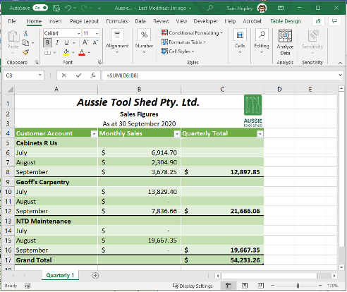
The following example shows a workbook containing some quarterly sales data for Aussie Tool Shed’s three main business customers.
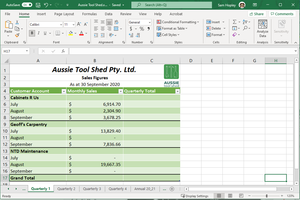
The total monthly sales are entered into quarterly sales reports. Suppose you were tasked to calculate the total annual sales for these business customers. To do this, you will first need to link cells within the same worksheet and then link cells between different worksheets.
Linking cells in the same worksheet
Your first step would be to compute the total quarterly sales for each of the three customers. You can do this by entering a SUM function in cells C8, C12 and C16 to total the monthly sales for each business customer. For example, you could enter the following function into C8:
=SUM(B6:B8)
Next, entering the following function into C17 would calculate the grand total for the quarter:
=SUM(C8,C12,C16)
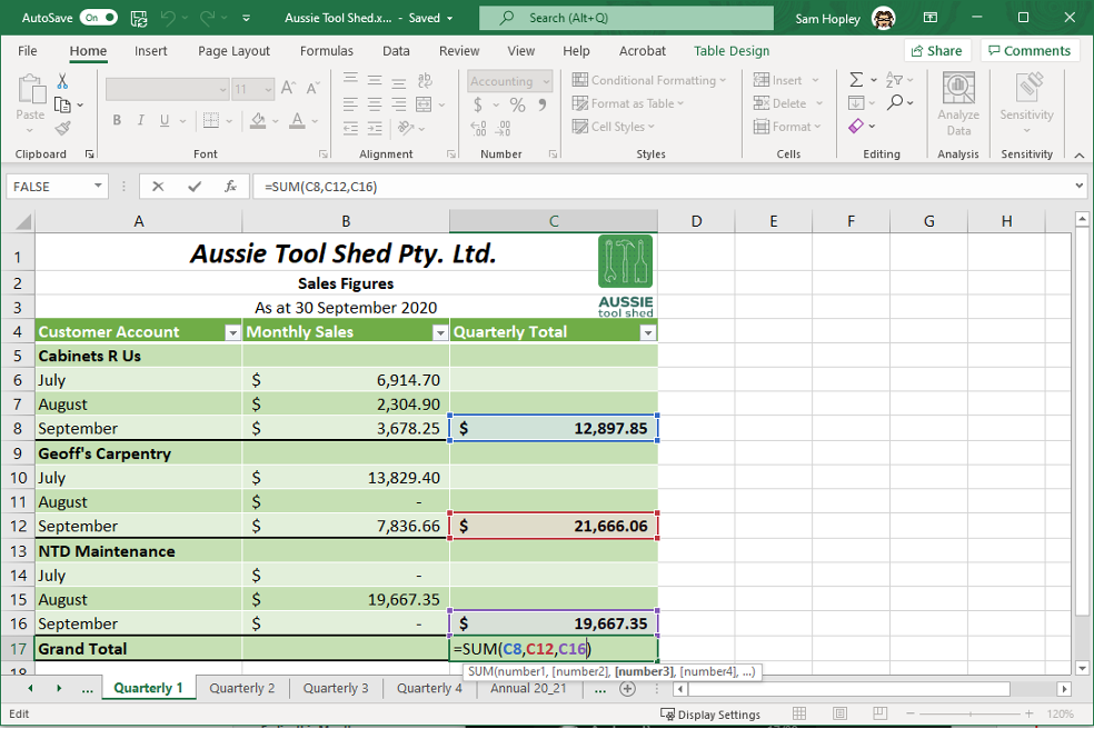
Using cell references instead of values in the function links the cells. If there are any changes to a referenced cell, the destination cell (the cell containing the cell reference) will automatically update accordingly.
For example, if a September sales total was added to the spreadsheet for ‘NTD Maintenance’, the ‘NTD Maintenance total’ (C16) would update, which would cause the ‘Grand Total’ (C17) to update as well. You wouldn’t need to recalculate anything!
Next, you need to calculate the annual total for each business customer. To do this, you will need to link different worksheets.
Linking cells from different worksheets
You would follow the same process to create a quarterly sales report for December, March and June. However, to create the annual sales report, you will need to reference the totals from each of the quarterly reports, which are on different worksheets.
To link cells on different worksheets:
- Start the function in the destination cell. In this instance, simply type the equals sign [=].
- Then click the appropriate tab to switch to the required worksheet.
- Next, click the cell you wish to reference.
- Press [Enter]. Excel will add the cell reference to the function.
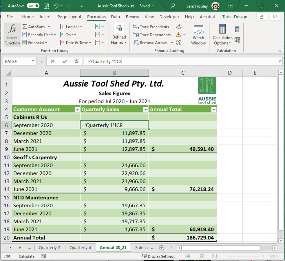
In this example, the formula in cell B6 is referencing the September sales total for ‘Cabinets R Us’. This information is located in cell C8 on the worksheet titled ‘Quarterly 1’. So, the formula that links the two worksheets is:
=’ Quarterly 1’!C8.’
If the referenced cell is edited, the destination cell on the linked worksheet will be automatically updated.
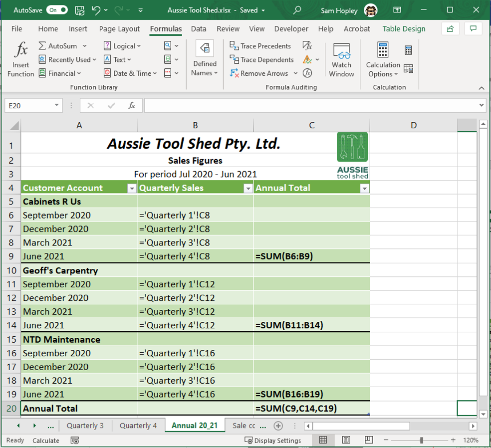
The same process applies to all the quarterly sales totals for each of the business customers. To see all the formulae in the sheet, press [Ctrl + `]. (The ` symbol (grave accent) is the key to the left of the number 1 in the numbers row on your keyboard.)
A formula that links worksheets within the same workbook has the following general syntax:
=‘WS’!X
Where:
- ‘…’! Indicates the cell reference is not on the same worksheet.
- WS is the name of the worksheet that contains the cell that you will reference.
- X is the cell reference in the reference workbook.
Linking cells from different workbooks
Suppose that when you were asked to create the annual sales report, the quarterly data was in separate workbooks rather than in separate worksheets within the same workbook. This time, to develop the annual report, you need to link cells from different workbooks.
To link separate workbooks, follow these steps:
- Click on the cell where you want the value from the other workbook to appear. In this case, B6.
- Type the equals sign [=].
- Go to the workbook with the worksheet containing the information you require. For this example, the ‘September Quarterly Sales Report’.
- Select the cell containing the data you want to show in the workbook where you are working. C8 shows the quarterly sales total for ‘Cabinets R Us’. Notice that your formula in the original worksheet has been updated.
- Press the [Enter] key to finalise your formula.
A formula that links workbooks has the following general syntax:
=‘[FN]WS’!X
Where:
- ‘…’! Indicates the cell reference is not on the same worksheet.
- [FN] is the file name of the reference workbook, including the file extension.
- WS is the name of the worksheet that contains the cell that you will reference.
- X is the cell reference in the reference workbook.
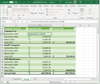
In this example, as shown in the previous images, the correct formula as shown is:
=‘[AussieToolShed_Sept.xlsx]Quarterly 1’!$C$8
Where:
- AussieToolShed_Sept.xlsx is the file name of the reference workbook.
- Quarterly 1 is the name of the referenced worksheet.
- $C$8 is the absolute cell reference of the required value.
Practice Exercise
Download the following Excel files and access the Cakes by Cloe practice exercise instructions to complete this exercise.
- Cakes by Cloe practice exercise instructions
- Cakes by Cleo North Excel File
- Cakes by Cleo South Excel File
- Cakes by Cleo West Excel File
- Cakes by Cleo East Excel File
After you have completed the practice exercise, you can check the sample answer here.

The following 4-minute video will help you better understand cells and the different operations regarding cells:
The following 4-minute video tutorial includes information on formatting cells, such as changing font size and colour, using bold, italic and underline commands, applying cell styles and changing text alignment:
Formatting Cells
Data attributes describe the properties that are unique to each cell in a spreadsheet. These attributes include:
- Formula – the formula or function contained within the cell.
- Value – the final, displayed value of the cell, which is computed after applying any formulae and functions within the cell.
- Format – the appearance settings applied to the value of the cell.
- Comments – any comments associated with the cell.
- Validation – any restrictions on the data or values that can be added to the cell.
When you develop your spreadsheet, consider how data attributes can be changed to meet the task requirements. We have already discussed formulae, functions and values. Let us now look at formatting in more detail.
The importance of formatting
When developing spreadsheets, it is often necessary to use multiple formats and formatting techniques across different cells. When planning your spreadsheet, consider the formatting task requirements. ‘What should your spreadsheet look like?
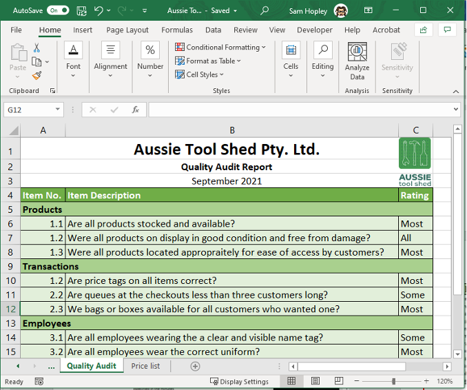
Different spreadsheets will have different formatting requirements depending on the purpose. Take a look at the following two examples:
Example 1:
Example 2:
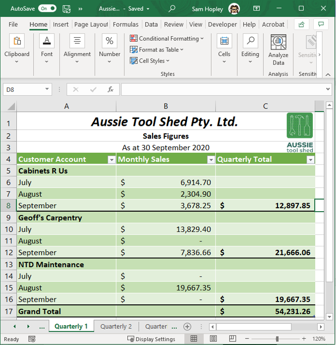
These two spreadsheets serve different functions, which means that they will have different sets of formatting requirements. For example, the spreadsheet in Example 1 uses different cell fill colours to group audit items together into categories to make them easier to locate. Meanwhile, the spreadsheet in Example 2 is used to report monetary values. It was formatted so that the decimal points line up, and the dollar symbols are displayed to clearly show that the data presented are monetary values. The total amounts were also emphasised by using boldface.
When formatting cells according to task requirements, always remember what data you are trying to report and figure out the best way to clearly report this data.
Key aspects of formatting
Spreadsheet formatting is important because it dictates how you will present your data. When you format a document, your goal is to ensure that the data you present is readable and understandable. This is why you input data into a spreadsheet in the first place. It helps you and other readers make sense of the raw data.
To ensure that the data on your spreadsheet is presentable and readable, there are three key formatting aspects to keep in mind:
- Accessibility
- Consistency
- Style.
Let us examine each of these aspects more closely.
Accessibility
Your spreadsheet must be formatted to be easily accessible and understandable by anyone who needs to read it. Think about your possible readers and ask, ‘What information will they look for?’. For example, if you develop a sales report that your supervisor will use to present the progress of the company to stakeholders, what information should you highlight? In this case, your supervisor would probably be most concerned with total figures. You could highlight the total figures in your spreadsheet by using boldface, a larger font or a different cell colour.
A well-formatted spreadsheet is easy to read and draws attention to the most appropriate information. On the other hand, a poorly formatted and inaccessible document would show little to no distinction among cells.
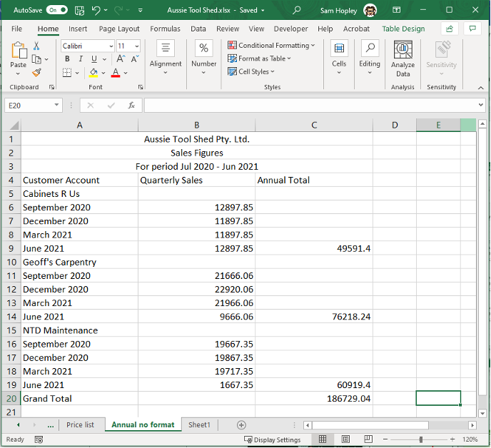
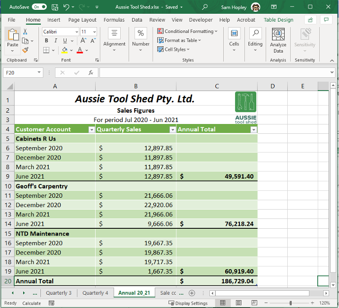
The data presented in the following two spreadsheets is the same. However, consider how the formatting of the second example's spreadsheet improves the accessibility of the information:
Example 1:
Example 2:
Consistency
Consistency of formatting applies when you create multiple similar workbooks. The best practice is that similar spreadsheets should follow a template that provides and highlights the same data each time. For example, the formatting of your monthly sales report for June must be consistent with that of May and previous months.
Regularly produced and referenced spreadsheets should be familiar. Changing the format every so often may confuse people who need to use your document. Automating formatting using macros or templates is the best way to ensure consistency. This will be discussed in the next topic.
Style
Your spreadsheets should also have some aesthetic similarities with other documents designed and produced by your organisation. When somebody outside your organisation reads your documents, they must be able to associate them with your organisation. This is why organisations have style manuals that detail the specific formatting and design guidelines to follow when producing documents. At the very least, most organisations will have a logo or a banner that should appear on every document or spreadsheet produced.
Here are some key aspects that you could implement during spreadsheet formatting and design to enhance presentation and readability:
1. It is important to choose the font carefully, according to the organisation's style guide. When selecting fonts, keep in mind the following:
- Select a clear font such as Calibri or Helvetica to present data.
- Limit the number of fonts used in a spreadsheet. Stick to one or two at most.
- Use a clear hierarchy of font sizes. Important texts, such as headers, should be larger than sub-headers. Subheaders should be larger than the data text.
2. When setting alignment, you control how data is displayed within a cell:
- Create a strong edge to spreadsheets by left-aligning all text data and right-aligning all numerical data. This improves readability and graphics consistency.
- Don’t use centre align as this causes the text to graphically “float” in the cell.
3. Spacing, shading, and gridlines all play a crucial role in enhancing the readability and visual appeal of a document
- Use white space to improve readability. Add white space to spreadsheets giving data additional room by adjusting column width and height. The vertical height of rows can also be increased to provide data with additional white space.
- Shade alternate rows to improve readability, for example, using a light grey.
- Use gridlines sparingly, and don’t place too much emphasis on the individual cell. For example, use a solid line for row borders and a dotted line for the column borders. Think of the gridlines as a guide for the reader’s eye.
4. Headers identify columns and rows of data within the spreadsheet:
- Define headers to make them clear and legible. Header text can be capitalised and bolded.
- 'Wrap Text' as needed to wrap data or headers around the cell.
5. Carefully consider a colour palette, for example, one or two colours that work well together.
6. Various appearances that can be applied to a cell or the text contained within it:
- Create cell styles for consistency; for example, in MS Excel, use the “New Cell Style” button to customise and name a new style.
- Use 'Conditional Cell Formatting'. This is useful if your spreadsheet contains a lot of data, as you can use conditional formatting to highlight important information in a worksheet and enhance the presentation.
This article explains 9 tips on how to improve your spreadsheet.
How to format a cell
When you format a cell, you are changing the appearance of the value contained in that cell.
You can format a cell or a range of cells. First, click a single cell or drag-select a range of cells. Next, right-click on your selection. Finally, choose the ‘Format Cells…’ option from the drop-down menu. Doing this will open the Format Cells dialogue box. You can also open this dialogue box by selecting the cell you want to format and pressing [Ctrl + Shift + F].
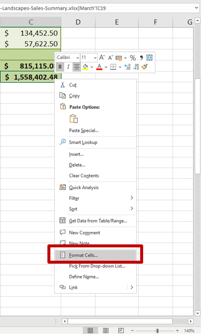
The Format Cells dialogue box has six tabs containing different formatting options. The six tabs are:
Let us discuss each of these formatting options further.
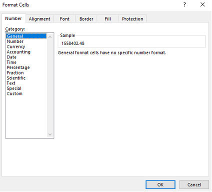
Number
The Number tab contains options relating to the way you can present numerical values. You can set the number format of a cell or group of cells based on the type of data you need to reflect.
The following 6-minute video explains number formatting.
Excel Numbers
For example, if you are working with sales figures, you should use the ‘Accounting’ format. Excel provides a brief description and a sample of the final formatted appearance for each of the options.
The following table outlines how the different number categories will format your data. In general, numerical values will be right-aligned in the cell. This means that the value will be positioned on the right side of the cell. Where an option asks you to specify the number of decimal places, Excel will automatically round to the number of decimal places specified or add zeros to the right of the number if required.
| Category | Description | Example output |
|---|---|---|
| General | Default number format. | 12345 |
| Number | Displays numerical values with the specified number of decimal places. | 123.40 |
| Currency | Displays general monetary values. | $ 123.45 |
| Accounting | Displays monetary values with currency symbols and decimal points lined up. | $ 123.45 $ 67.80 |
| Date | Displays date values in the specified format. | 30/06/2021 |
| Time | Displays time values in the specified format. | 12:00:00 AM |
| Percentage | Multiplies the cell value by 100 and adds a percentage symbol and the number of decimal places you specify. | 12% |
| Fraction | Displays the cell value as a fraction | 1/8 |
| Scientific | Displays the cell value in scientific notation, where the ‘E’ represents ‘×10 to the power of’. | 1.20E-01 |
| Text | Treats the content of the cell as text even if a number is entered and positions the value to the left side of the cell. | 0.12 |
| Special | Special number formats depending on your location (as of writing, there are no special formatting options that apply to Australia). | N/A |
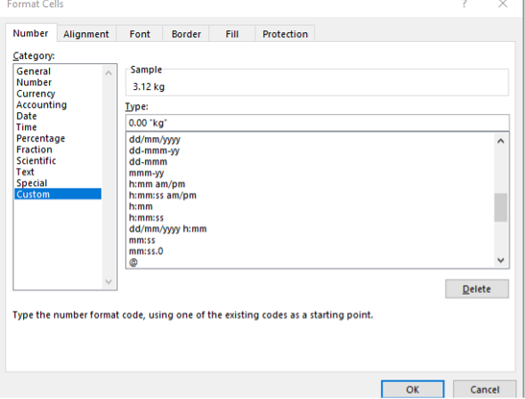
Custom number formats
You can also use the Number tab to design custom formats. This allows you to use formatting codes to express your data in formats not specifically built into Excel. You can also edit existing number format pre-sets to better suit the data you want to present. This is a very powerful tool and gives you a great deal of control over the way Excel displays your numerical data.
For example, imagine you are developing a spreadsheet for Aussie Tool Shed that records the weight of large tools for shipping and storage purposes. You want your data to display numbers up to two decimal places, followed by ‘kg’ as the unit of measurement. To achieve this:
Using this custom formatting, a data entry, ‘3.124’, will now be displayed as ‘3.12 kg’.
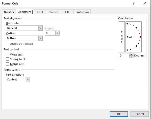
Alignment
The settings found here allow you to modify the positioning of text found inside the cell. You can set the following:
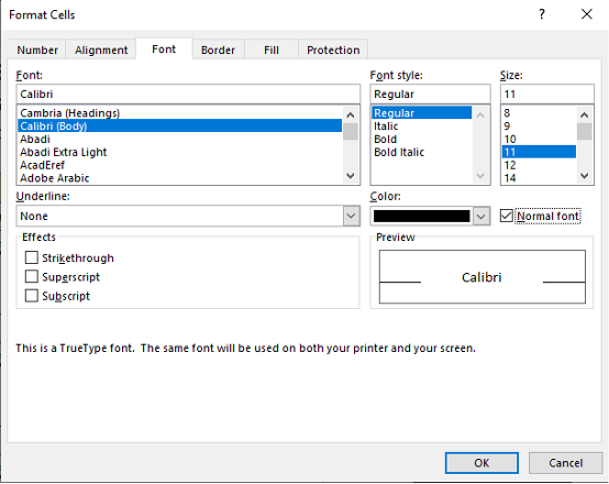
Font
This tab allows you to control the font settings for the cell. You have the following options:
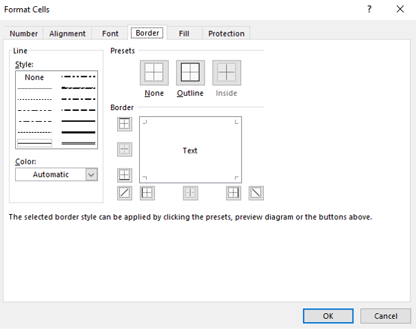
Border
This tab gives you complete control over the borders around and between cells in your selection. You have the following options:
When selecting line positions, they will relate to the cell or range of cells you have selected. When you select more than one cell, you can choose to place borders around just the outside of your selection or between the cells within the selection.
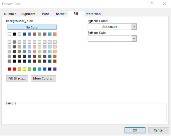
Fill
This tab allows you to set the background properties of the cells selected. You have the following options:
Protection
The protection tab gives you options to lock or hide cells in conjunction with the worksheet protection options available in Excel.
Locked cells appear and function as normal, but you require a password to edit them.
Hidden cells appear to be empty. However, if you have the correct access requirements, you can still see and edit the hidden cell in the formula bar. Hidden cells are a great way to hide confidential information, such as personal information.
To use locked or hidden cells, you must protect the worksheet first. Protecting a worksheet prevents editing. Using the locked cell formatting, you can control which parts of the sheet can and can’t be edited by other people.
The following 4-minute video explains how to protect a worksheet.
Protecting a sheet in Excel
Copying and pasting data attributes
Remember that the data attributes of a cell in a spreadsheet include:
When you format cells, you can use attributes from one cell and apply them to other cells instead of manually setting the formatting for each cell. To do this, follow these steps:
You can also double-click the ‘Format Painter’ button to toggle the function on. Now it will paste the attributes into any cells you select until you either click the ‘Format Painter’ button again or press the [Esc] key.
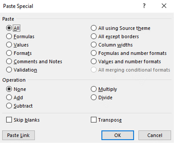
While the ‘Format Painter’ is useful, it always copies all the attributes to the destination cells. The ‘Paste Special’ tool allows you to select which attributes to copy and which to ignore.
Anytime you have the contents of a cell (or selection of cells) copied to the clipboard, you can right-click on a selection of other cells and select ‘Paste Special’ from the drop-down menu. This opens the ‘Paste Special’ dialogue box, which gives you the option to copy some or all the copied cells’ attributes to the selected cells.
For example, by using ‘Paste Special’, ‘Values’, you can copy the calculated value from a cell containing a formula without copying the formula itself.
Cell referencing
When developing spreadsheets, it is often useful to reference the data in one cell of the spreadsheet to use it as part of a formula or function in another cell. This can be done in two ways, relative cell referencing or absolute cell referencing.
Relative cell referencing
Relative cell referencing is the default form of cell referencing in Excel. When you copy a relative cell reference and paste it into a different cell, the referenced cell changes relative to the location of the new destination cell. In other words, the direction and number of cells between the reference cell and destination cell remain the same, but the actual cell locations shift.
For example, if you reference cells A1 and B1 in cell C1 using the formula, =A1+B1. The referenced cells and destination cells are in the same row, one column apart. If you copy this (relatively referenced) formula from C1 down to C3, you will get the formula =A2+B2 in C2 and =A3+B3 in C3.
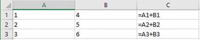
This relative referencing has shifted relative to where it was copied from and where it was copied to. The referenced cells and destination cells are in the same row, one column apart. As you shifted one row down when copying it, the referenced cells A1 and B1 were shifted down one row as well so that the new formula in C2 referenced cells A2 and B2. This then continued as you shifted down another row to C3.
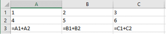
The same thing happens if you copy across a row. The relative referencing tracks the relative position of the cells.
Absolute Cell Referencing
Absolute cell referencing is different. It is used when you want the cell reference to stay fixed on a specific cell, row or column, regardless of where it is copied.
Absolute referencing is specified by using $ symbols before the column letter and/or row number. If you were to use absolute referencing in the previous example (by changing the formula to =$A$1+$B$1), you would get a different result, as shown in the following image.
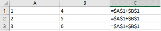
This time, the cell references do not shift when you copy the formula to different cells; they are fixed on cells A1 and B1 specifically due to the use of the $ signs in the formula. So, no matter where you copy it, the formula will always be =$A$1+$B$1.
You have three options when using absolute cell referencing: you can use absolute row referencing, absolute column referencing, or absolute row and column referencing.
When using a partial absolute reference, the absolutely referenced row or column stays fixed, but the relatively referenced row or column shifts relative to where it is copied from and to.
You can turn a relative cell reference into an absolute cell reference by typing $ symbols into the formula or function. You can also click on the relative cell reference in the function bar and press [fn + F4]. This automatically adds the $ symbol to both the column and row references.
When using cell references in formulae and functions, it is important to test them to make sure they actually compute the data required by the spreadsheet task. This is particularly important when you are developing linked spreadsheets.
The following 9-minute video tutorial demonstrates cell referencing.
Practice Exercise
Download the following Excel file: ABC Pty Ltd – Practical Exercise
Using Absolute references, calculate:
After you have completed the practice exercise, you can check the answer here.
- Various appearances can be applied to a cell or the text contained within it:
- Create cell styles for consistency; for example, in MS Excel, use the “New Cell Style” button to customise and name a new style.
- Use “Conditional Cell Formatting”. This is useful if your spreadsheet contains a lot of data, as you can use conditional formatting to highlight important information in a worksheet and enhance presentation.
- Number
- Alignment
- Font
- Border
- Fill
- Protection.
- Select the cells you wish to format.
- Open the ‘Format Cells…’ dialogue box.
- Click the ‘Custom’ category.
- Enter the following in the ‘Type’ text field:
- The number format with the desired number of decimal places (for this example, 0.00).
- The unit of measurement is displayed as text, enclosed in double quotation marks (For this example, “kg”)
- Horizontal alignment – adjusts the position of the value from left to right.
- Vertical alignment – adjusts the position of the value up and down.
- Indentation – adjusts the space between the value and the edge of the cell.
- Orientation – adjust the angle of the text.
- Text control – changes the way the cell responds to the value within it
- Wrap text – automatically breaks long text into multiple lines to fit inside the width of the cell. The row height automatically adjusts.
- Shrink to fit – automatically reduces the size of the font so that the value fits inside the width of the cell.
- Merge cells – joins two or more consecutive cells together into a single large cell.
- Text direction – adjusts text to be read from lift to right or right to left.
- Font - change the style of writing, add italics, bold or both.
- Underline – add different types of underlining.
- Colour – change the colour of your text.
- Font effects – strikethrough, superscript or subscript.
- Normal font – selecting the normal font check box resets the font, font style, size, and effects to the normal (default) style.
- Line style
- Line colour
- Line positions – top, bottom, left, right, diagonal, horizontal and vertical borders.
- Fill colours
- Fill effects
- Fill pattern colours
- Fill pattern styles.
- Formula
- Value
- Format
- Comments
- Validation.
- Select the source cell – the cell that contains the attributes that you want to copy. For example, 10C.
- Click the ‘Format Painter’ button, which can be found on the ‘Clipboard’ category of the ‘Home’ tab of the ribbon.
- Select the destination cell or cells – the cell or cells you want to apply the attributes to. In this example, the cell fill colour, bolding and financial formatting are applied to C12.
- $A1 is absolute referencing column A but relative referencing row 1.
- A$1 is relative referencing column A but absolute referencing row 1
- $A$1 is absolute, referencing both column A and row 1.
- The % of total sales for each salesperson
- The commission earned by each salesperson for Qtr. 4 2023
-
Spacing, shading, and gridlines all play a crucial role in enhancing the readability and visual appeal of a document:
- Create a strong edge to spreadsheets by left-aligning all text data and right-aligning all numerical data. This improves readability and graphics consistency.
- Don’t use centre align as this causes the text to graphically “float” in the cell.

As with any document, errors are possible when using formulae and functions – either through ‘typos’ or through incorrect applications of syntax. This follows the ‘GIGO’ principle (Garbage In, Garbage Out), which states that your output data quality is only as good as the data that is entered into the formula.
It is important to test each formula you incorporate into a spreadsheet to confirm that the data output from the formula meets the expected output and the task requirements.
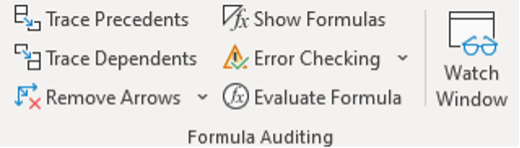
Excel offers multiple ways to test that your formula is meeting task requirements. These can be found on the ‘Formula Auditing’ group of the ‘Formulas’ tab on the ribbon.

The following options can be found in the ‘Formula Auditing’ group and will be discussed in more detail:
- Trace Precedents
- Trace Dependents
- Remove Arrows
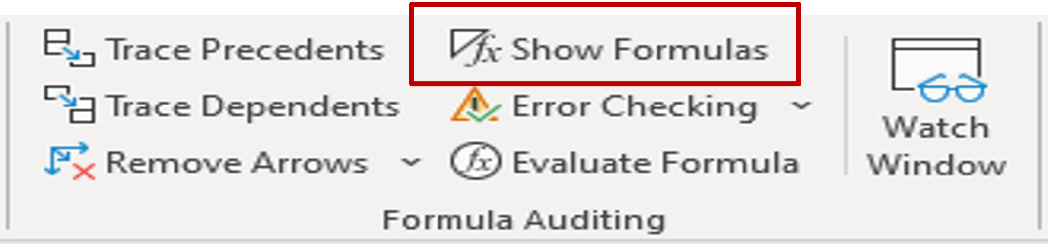
- Show Formulas
- Error Checking
- Evaluate Formula
- Watch Window
Trace precedents and dependents
The ‘Trace Precedents’ and ‘Trace Dependents’ buttons are ways for you to check how the formulae in your worksheet are connected to each other.
A precedent cell is a cell that is referenced in a function or formula in another cell. The cell precedes or is populated before the dependent cell.
A dependent cell is a cell that contains a function or formula that references other cells. The value in this cell depends on the value in the precedent cell.
The precedents and dependents are shown through arrows connecting different cells.
How to trace precedents
To trace the precedents of a cell, follow these steps:
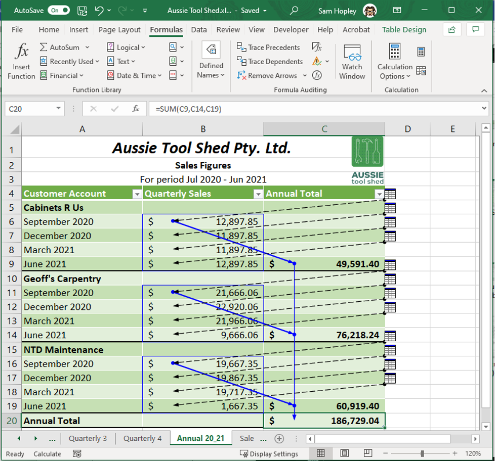
- Select the cell containing the formula that you want to trace. For example, if you want to trace the precedents of C20, select C20.
- Click the ‘Trace Precedents’ button. Arrows will appear, pointing from the cells needed to compute the value in your selected cell.
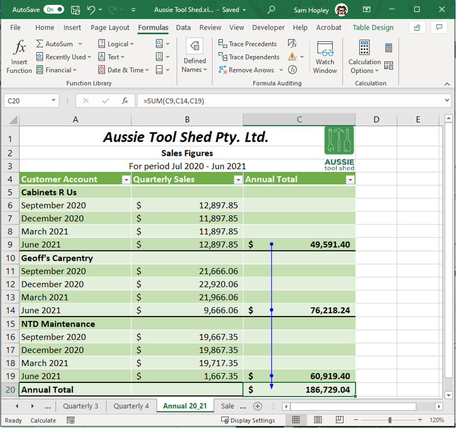
In this example, you can see that C9, C14 and C19 are precedents for C20, as indicated by the blue dots and arrows. - Click the ‘Trace Precedents’ button again. This will show the next level of cells that are connected to your selected cell. You can click the ‘Trace Precedents’ button repeatedly until all levels of precedents related to your selected cell are shown.
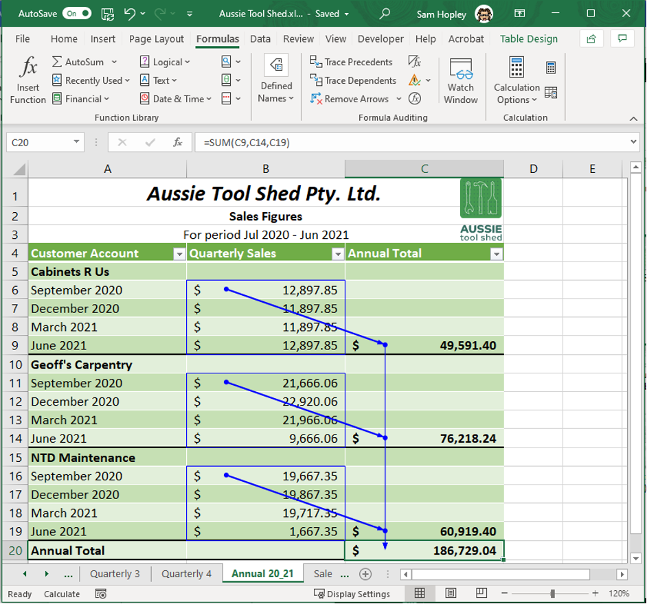
In this example, Excel shows that the cells in the range B6:B9 are precedents for C9 by placing the range in a blue box. In the same way, B11:B14 are precedents for C14, and B16:19 are precedents for C19.
A third click of ‘Trace Precedents’ reveals that all of the values in column B also have precedents. However, these precedent cells are located on a different worksheet. This is indicated by dashed, black arrows and the spreadsheet icons.
How to trace dependents
A similar process can be followed when tracing dependents:
- Select the cell with dependents that you want to trace. For example, if you want to trace the dependents of cell B6, select B6.
- Click the ‘Trace Dependents’ button. You will see blue lines coming from your selected cell pointing toward all the dependents of that cell.
In this example, the blue arrow indicates that C9 is a dependent of B6. - Click the ‘Trace Dependents’ button again to show the next level of dependents. You can click this button repeatedly until all levels of dependents related to your selected cell are shown.
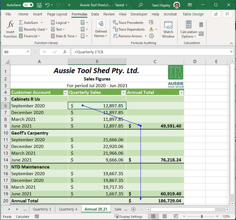
If any dependents are located on a different worksheet, they will be indicated by a dashed black arrow and the spreadsheet icon.
Tip: If precedent or dependent cells are in another workbook, that workbook must be open for Excel to include in tracing.
The following 3-minute video explains formula auditing in Excel.
Trace all cell relationships
Excel also allows you to trace all relationships in your active sheet at once. To do this:
- Type the equals sign [=] into an empty cell, near but not a part of the table that contains your data.
- Click the ‘Select All’ button – the diagonally shaded square found in the top left corner between the column and row labels. Excel will highlight all the cells in your current sheet and enter ‘=1:1048576’ into your selected cell.
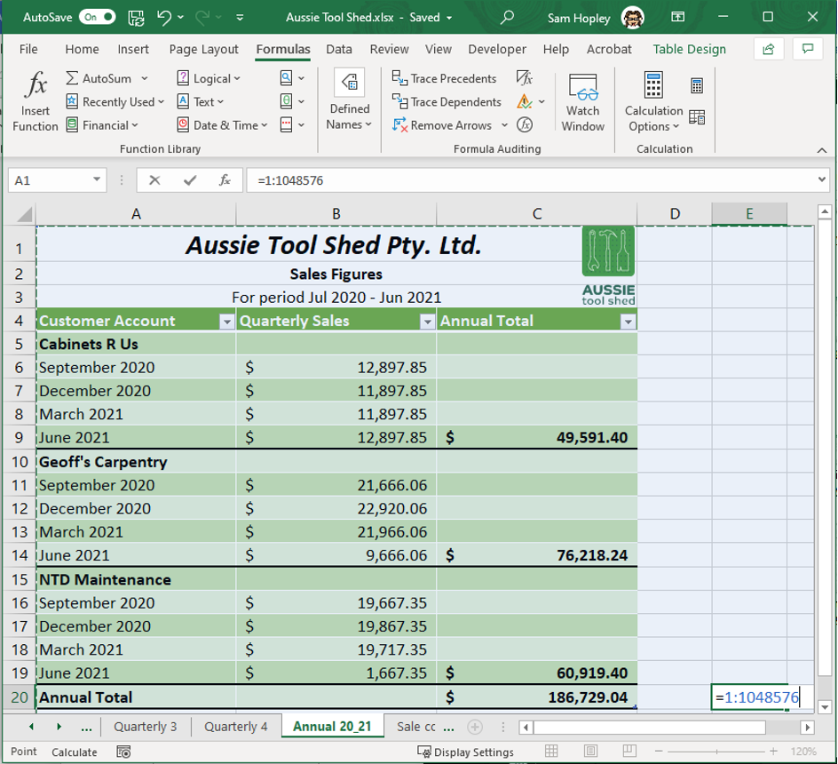
- Click the ‘Tick icon’ in the ‘Formula Bar’. You may see a popup warning you that Excel cannot evaluate the formulas. Click ‘OK’. The cell value will now show as a ‘0’.
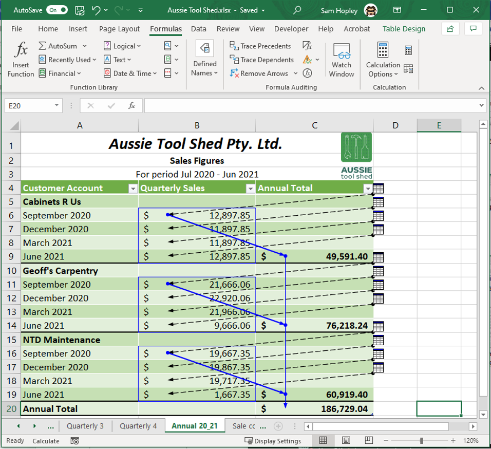
- Make sure the ‘0’ cell is selected. Click the ‘Trace Precedents’ button twice. This will show all relationships in your active sheet. Delete the contents of the ‘0’ cell.
Once you are finished tracing the precedents and dependents of your worksheet, you can clear the arrows from the screen by clicking the ‘Remove Arrows’ button from the ‘Formula Auditing’ category of the ‘Formulas’ tab on the ribbon. You can also opt to remove only the precedent arrows or only the dependent arrows by clicking on the drop-down menu.
By making it a habit to trace precedents and dependents, you can ensure that the functions and formulae in your spreadsheet reference the correct cells. As a result, you are also assured that your spreadsheet output meets the task requirements.
In the example used here, you know that your quarterly and annual sales figures for Aussie Tool Shed are accurate because you were able to trace the cell references that were used to calculate the total values.
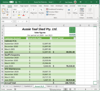
Show formulas
Another feature found in the ‘Formula Auditing’ category is ‘Show Formulas’, which was discussed briefly earlier in this topic. Clicking this button will show you all the functions and formulae used in the current worksheet. These functions and formulae will be displayed in the respective cells that contain them.
As with tracing precedents and dependents, you can use the ‘Show Formulas’ button to view all of the functions and formulae and confirm they are correct. Aspects of functions and formulae to check include whether:
- the syntax is correct for each function and formula
- the correct cells or cell ranges are used in each function and formula.
By doing so, you can ensure that the values in your spreadsheet will be computed and displayed correctly according to task requirements.
Error checking
Excel cannot compute functions and formulae if they contain errors in the following:
- syntax
- arguments
- cell references.
When Excel cannot compute a value, it will display an error code instead to let you know there is a problem. Error codes include:
- #DIV/0!
- #N/A!
- #NAME?
- #NULL!
- #NUM!
- #REF!
- #VALUE!
You do not need to learn what the different error codes mean. However, you should be able to recognise an error code in order to locate a function or formula that needs to be fixed.
The ‘Error Checking’ tool uses rules that help check formulae in your spreadsheets for errors. The ‘Error Checking’ button is located in the ‘Formula Auditing’ category of the ‘Formulas’ tab.
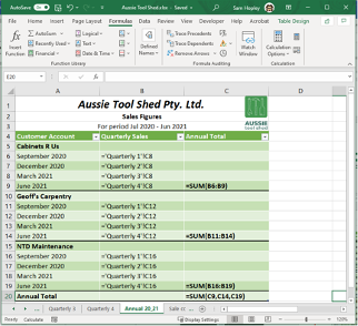
There are three different ways in which you can check errors in your spreadsheet. Excel provides you with the following options under the ‘Error Checking’ drop-down menu:
- Error Checking
- Trace Error
- Circular References
Error checking
If your worksheet contains any errors, clicking the ‘Error Checking’ button will display the ‘Error Checking’ dialogue box, as shown in the following example.
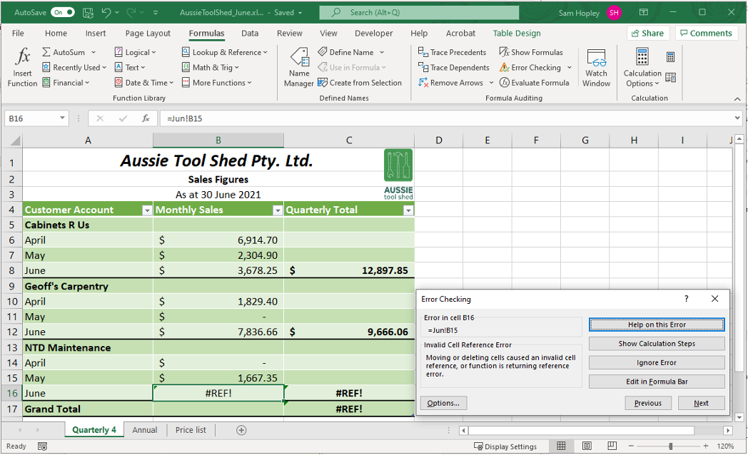
This dialogue box will show you which cells contain errors, which formulae are involved and a brief description of the error. From here, you can select one of the following buttons to resolve the error:
- ‘Help on this Error’ – This will launch the Microsoft Support website, which will give you information and examples based on the error code.
- ‘Show Calculation Steps’ – This will open the ‘Evaluate Formula’ dialogue box. Here you can see, step-by-step, how Excel calculated the formula you entered and identify the step(s) where the error occurred.
- ‘Ignore Error’ – This removes the error tag on the cell so that it does not appear in future error checks.
- ‘Edit in Formula Bar’ – This redirects your cursor to the formula bar so that you can manually edit your formula.
If there are multiple errors on one spreadsheet, you can inspect and fix each of them by clicking ‘Next’ and ‘Previous’ in the ‘Error Checking’ dialogue box.
Trace error
To use the ‘Trace Error’ function, select a cell that contains an error, then click the ‘Trace Error’ button. Excel then displays arrows that show you which cells caused the error value on your selected cell. From the arrows in the following example, you know that B16 caused the error on C16, which, in turn, caused the error on C17.
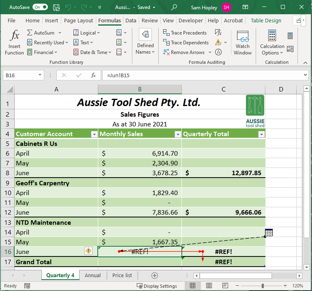
You can use the ‘Remove Arrow’ to remove the error traces when you are finished.
Circular references
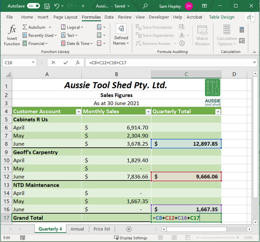
A circular reference happens when a formula references the cell it is entered into.
The following image shows an example of a circular reference. The formula is entered on C17. Notice, however, that C17 is also part of the formula. In this case, Excel will not calculate a final value. Instead, it will tag this as a circular reference, and you may see an error warning popup.
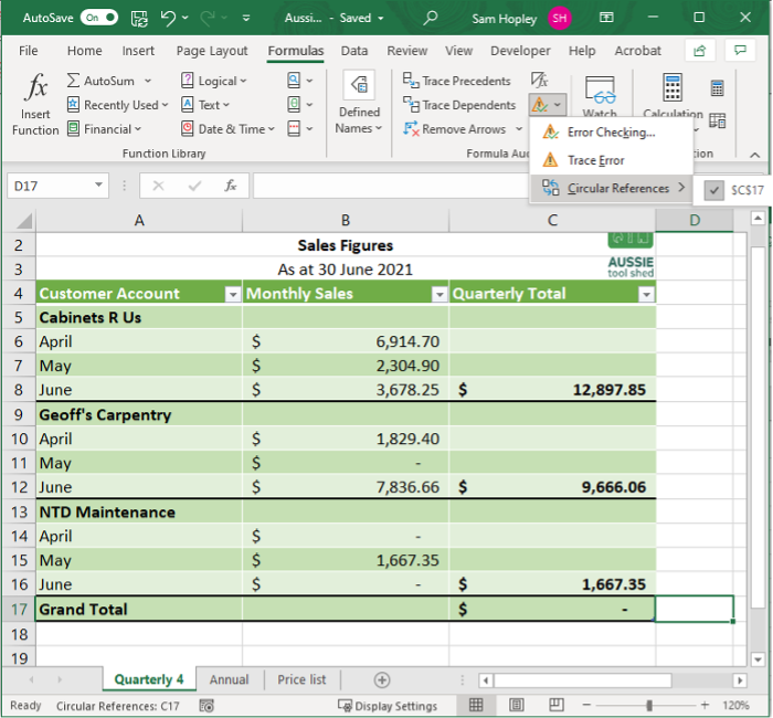
You can check your spreadsheet for circular references by going to the drop-down menu of the ‘Error Checking’ button and clicking on ‘Circular References’. A list of cells containing circular references will be displayed, as shown in the following image.
Error checking to confirm output meets task requirements
There are two (2) main types of errors in spreadsheets:
- Errors that prevent the spreadsheet software from performing the computation will display an error code instead of a value.
- Errors that can be computed but do not produce the correct value because they contain a typing mistake or reference the wrong cell can be trickier to locate.
Tracing precedents and dependents will help you identify these types of errors.
Performing regular error checks will help you ensure that all values contained in cells are correct. Errors can affect multiple cells or entire worksheets and workbooks if not identified and corrected. When you encounter errors in your document, use the error-checking tools available in the spreadsheet software to help you fix them. By doing so, you can ensure that the functions and formulae in your spreadsheet result in accurate values. This means that your spreadsheet output, as a whole, is also an accurate document that addresses the task requirements.
Evaluate formula
The ‘Evaluate Formula’ tool in the ‘Formula Auditing’ category on the ‘Formulas’ tab of the ribbon of Excel walks you through the steps used in testing a result from a formula. This helps locate errors in long formulae or those that have multiple levels of precedents.
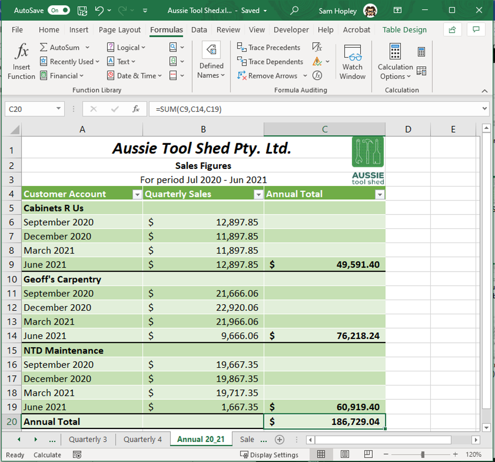
As an example, say you wanted to evaluate the formula used in C20 to calculate the annual sales total for Aussie Tool Shed’s business customers. When you select C20 and click ‘Evaluate Formula’, the ‘Evaluate Formula’ dialogue box will appear.
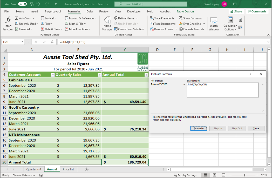
In the dialogue box, you will see the absolute cell reference on the left side and the evaluation box on the right. The evaluation box will first show you the initial formula that you entered in that cell. In the previous example, you can see the initial formula, =SUM(C9, C14, C19), appears inside the evaluation box.
Clicking the ‘Evaluate’ button repeatedly will walk you through the steps that Excel used to arrive at the final value using the formula that you entered. When the evaluation is finished, you will see that the ‘Evaluate’ button will be replaced with the ‘Restart’ button, which you can click to evaluate the formula from the beginning.
You will notice that certain parts of the formula are underlined for each step in the evaluation. This means that there are other functions or formulae nested in that part of the formula. In the following example, B6 is underlined. This means that B6 contains another formula. You can check and evaluate this formula separately by clicking on the ‘Step In’ button.
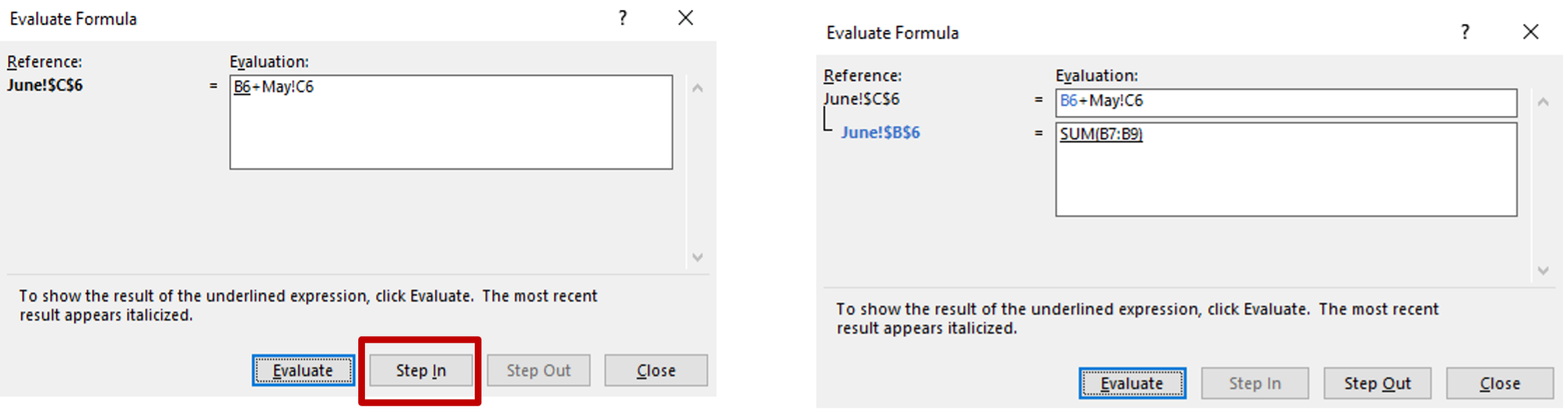
In this example, the image on the right shows that B6 contains the function =SUM(B7:B9).
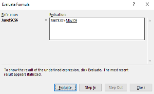
Clicking the ‘Step Out’ button will return you to the original formula, now with the nested formula evaluated, as shown in the following image.
As you use more complex functions and formulae in your spreadsheets, you will realise the importance of evaluating formulae. There may be times when you need to reference an existing function or formula in a new function or formula. This is called ‘nesting’. The ‘Evaluate Formula’ button will help you spot any errors or inconsistencies that come from nested functions or formulae. By evaluating formulae, you can ensure that the functions and formulae you have entered are calculating the correct values, even as you add more data to your spreadsheet. This means that the computations in your spreadsheet will always produce output according to task requirements.
The following 21-minute video explains 5 tips to evaluate advanced formulas in Excel:
Evaluating formula with F9
Additionally, the F9 key serves as a powerful tool for debugging formulas and conducting interactive scenario analysis.
To evaluate a formula in Excel using the F9 key, follow these steps:
- Select the cell: Click on the cell containing the formula you want to evaluate.
- Enter edit mode: Press F2 to enter the cell's edit mode. This allows you to see and edit the formula directly within the cell.
- Highlight the part of the formula: Using your mouse or keyboard, highlight the specific part of the formula you want to evaluate. If you want to evaluate the entire formula, skip this step.
- Press the F9 key: With the part of the formula highlighted, press F9. Excel will replace the selected portion with its calculated result.
- Review the result: Observe the result displayed in the formula. This helps in understanding how Excel processes that part of the formula.
- Undo the evaluation (Optional): If you want to revert to the original formula, press Ctrl + Z immediately to undo the change and restore the formula.
- Exit edit mode: Press Enter to exit edit mode and retain any changes, or press Esc to exit without saving changes.
The following 3-minute video demonstrates how to use F9 for evaluating formulas:
Watch window
The ‘Watch Window’ tracks the changes in the value of a particular cell. This is a convenient tool to use when you are working with multiple spreadsheets at the same time or spreadsheets with many rows and columns that do not fit into the current view on your screen.
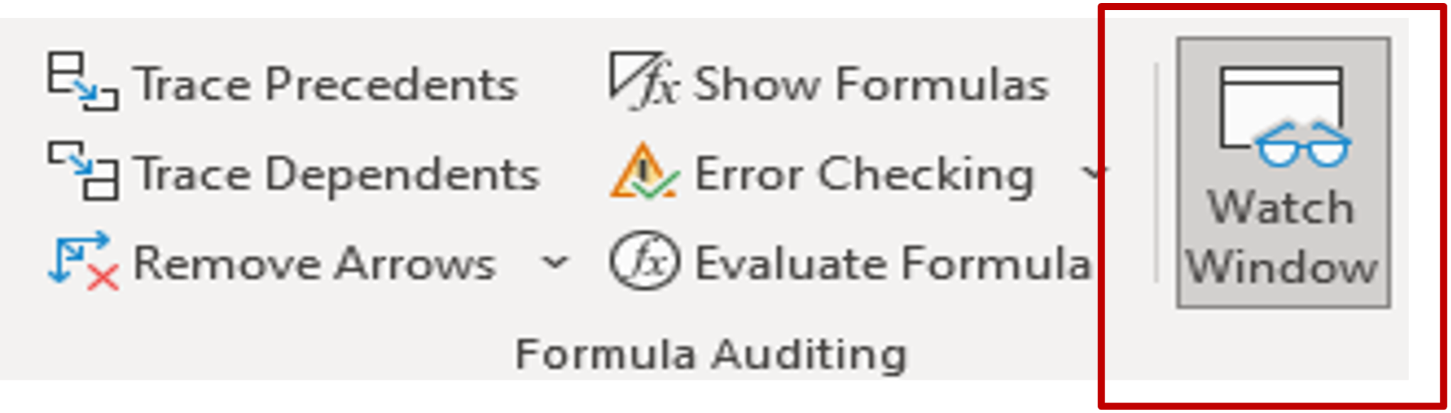
The following image shows an example of a ‘Watch Window’. From this window, you know that you are tracking cell C20. The ‘Watch Window’ gives you information on the workbook title, worksheet title, cell name, cell reference, value and formula. Any changes you apply to the cell will be updated on the watch window.
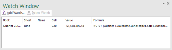
You may track multiple cells in the same window by clicking on the ‘Add Watch’ button. You may also delete a watch if you no longer need it.
The ‘Watch Window’ will be open and visible even if you open new worksheets or workbooks. You can use this to keep track of cells that hold critical data and formulae and make sure that they do not result in errors as you edit your spreadsheet. The ‘Watch Window’ is a useful tool for tracking cells that contain values that change regularly as you enter data.
For example, if your spreadsheet output will display multiple total values, it would be helpful to track these totals in the watch window. That way, you can easily check if the totals are correctly updated as you add more data. By doing this, you can ensure that the spreadsheet output contains accurate data and meets task requirements.
Practice Exercise
Download the following Excel file and the Sportique Pty Ltd practice exercise instructions to complete this exercise.
After you have completed the practice exercise, check the answer here.
For this activity, you will create your first spreadsheet, an Aged Debtor Report. Through this activity, you will demonstrate your ability to use basic design features to enhance the readability and appearance of the spreadsheet
To begin with this task, carefully follow the steps below:
- Open Microsoft Excel
- Open a new workbook
- Save the workbook as ‘BSBTEC402 –Design and Produce Complex Spreadsheets –Spreadsheet 1 Aged Debtor Report’
- In cell A1, write the title of the workbook as ‘Aged Debtor Report A-5’
Copy and paste the contents of the report (Aged Debtor Report - CBSA) into the spreadsheet from cell A2 onwards
Format the text so that it contains:
- The same colour scheme (look at the extract below)
- Arial font–Size 10
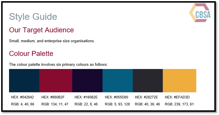
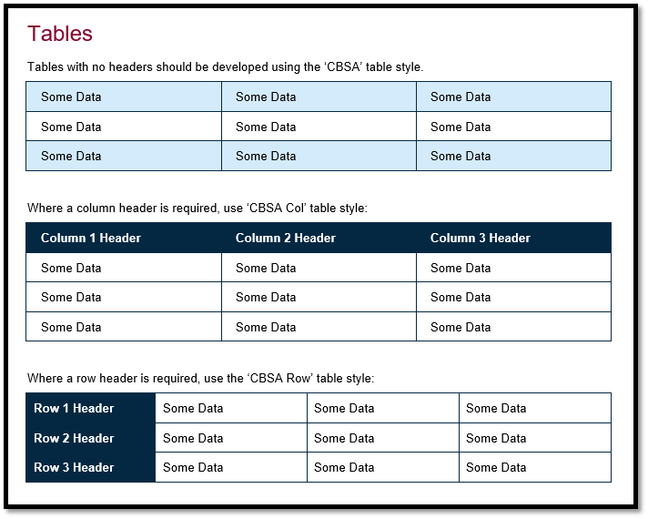
- Format the ‘Aged Debtor Report A-5’ heading so that it is bold
- Adjust the rows to size 25▪Adjust the columns to fit the text
- Right-click on the worksheet tab at the bottom of the document, currently titled ‘Sheet 1’ and rename the tab ‘Aged Debtor Report A-5’
- Save your work (it is good practice to do this as you go)
Learning Checkpoint Answer
This is an example of how your spreadsheet should look: